Lesson 36 Transformations

Motivating Example

You buy fencing for a square enclosure. The length of fencing that you buy is uniformly distributed between 0 and 4 meters. What is the distribution of the area of the enclosure?

Most people realize that the area must be between 0 and 1 square meters, since the length of each side must be between 0 and 1 meters, and the square of a number between 0 and 1 is also between 0 and 1. But how likely are the values in between?

Theory

We can formalize the above example as follows. The length of fencing, \(L\), is a \(\text{Uniform}(a=0, b=4)\) random variable, and we are interested in the distribution of \(A = (L/4)^2\).

First, let’s simulate the distribution of \(A\). The Colab below begins with a uniform random variable \(L\), defines \(A = (L / 4)^2\), and displays 10000 simulations of both \(L\) and \(A\).

In the simulation above, \(L\) is equally likely to take on all values between 0 and 4. This is not surprising because \(L\) was defined to be this way (a uniform distribution between 0 and 4). The distribution of \(A\) is more interesting. It is much more concentrated toward the lower values than the higher values. In hindsight, this makes sense because \((L / 4)\) is a number between 0 and 1, and numbers between 0 and 1 get smaller when we square them.

How do we derive the p.d.f. of \(A\)? This is a special case of a more general problem. We have a random variable \(X\) whose distribution we know, and we want to find the distribution of \(Y = g(X)\), a transformation of \(X\). The strategy for these problems is this:

1. Calculate the c.d.f. of \(Y\) (by rewriting the event in terms of \(X\) and using the known distribution of \(X\)).
2. Take the derivative to obtain the p.d.f. of \(Y\) (by Definition 33.2).

Example 36.1 Let’s apply this strategy to the example at the beginning of the lesson.

First, we find the c.d.f. of \(A\), the area of the enclosure. We write out the definition of the c.d.f., express \(A\) in terms of \(L\), and rearrange the expression to make the probability easy to calculate. \[\begin{align*} F_A(x) &= P(A \leq x) \\ &= P\left((L/4)^2 \leq x\right) \\ &= P(L \leq 4 \sqrt{x}) & \text{(if $x \geq 0$)} \\ &= \begin{cases} 0 & x < 0 \\ \sqrt{x} & 0 \leq x \leq 1 \\ 1 & x > 1 \end{cases}. \end{align*}\]

Now we take the derivative to get the p.d.f. \[ f_A(x) = \frac{d}{dx} F_A(x) = \begin{cases} \frac{1}{2\sqrt{x}} & 0 \leq x \leq 1 \\ 0 & \text{otherwise} \end{cases}. \]

We graph the p.d.f.s of \(L\) and \(A\) below. Compare these with our simulations above.

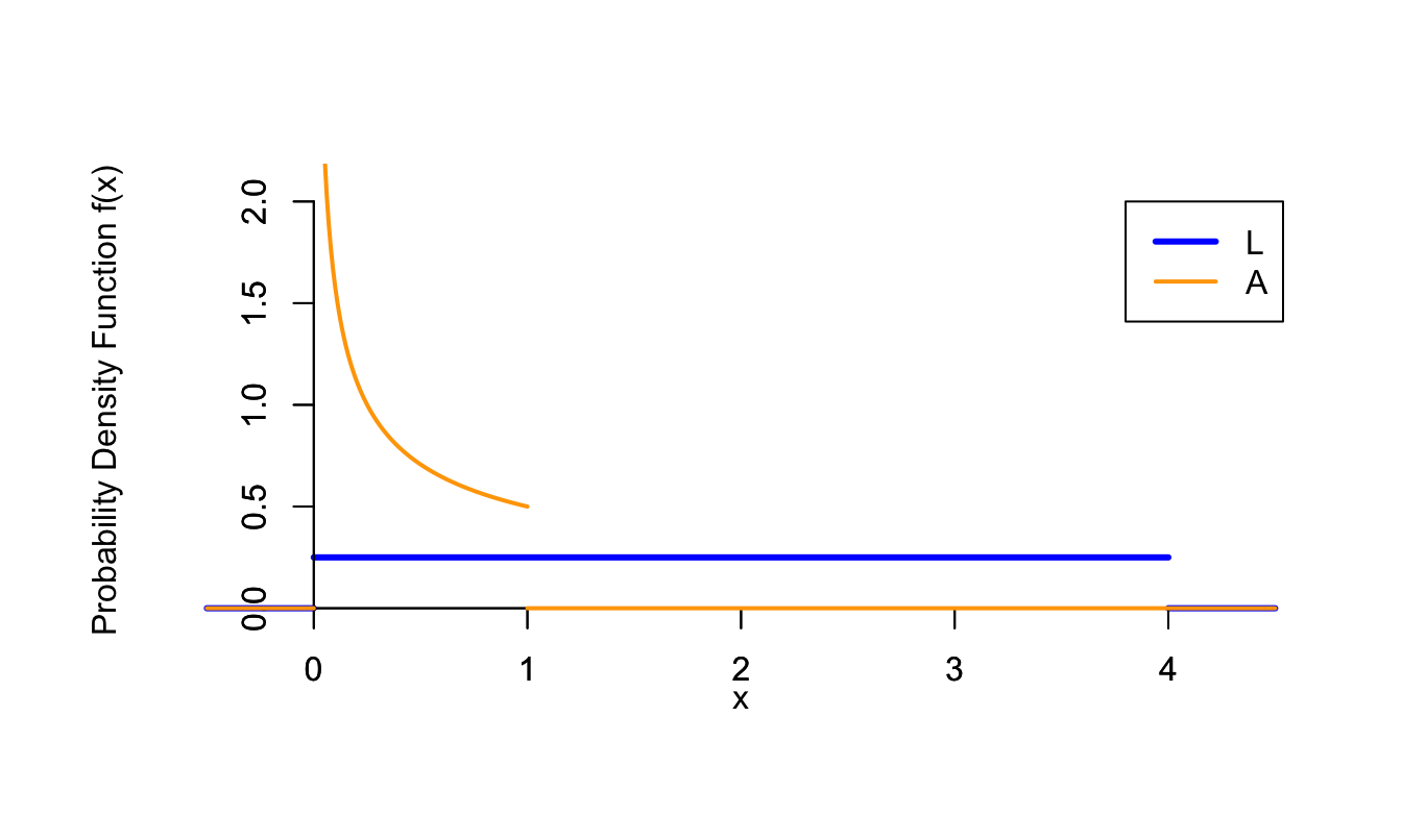
Figure 36.1: Distributions of \(L\) and \(A\)

Now, we derive formulas for the two most common types of transformations: shifting by a constant and scaling by a constant.

Theorem 36.1 (Shift Transformation) Let \(X\) be a continuous random variable with p.d.f. \(f_X\). The p.d.f. of \(Y = X + b\) is \[\begin{equation} f_Y(y) = f_X(y - b). \tag{36.1} \end{equation}\]

Proof. We can express the c.d.f. of \(Y\) in terms of the c.d.f. of \(X\): \[\begin{align*} F_Y(y) &= P(Y \leq y) \\ &= P(X + b \leq y) \\ &= P(X \leq y - b) \\ &= F_X(y - b). \end{align*}\]

Taking the derivative, we see that the p.d.f. is \[ f_Y(y) = \frac{d}{dy} F_Y(y) = f_X(y - b). \]

The figure below illustrates a hypothetical p.d.f. for a random variable \(X\) and the corresponding p.d.f. for the shifted random variable \(Y = X + 1\). Notice how the p.d.f. is exactly the same, except shifted to the right by 1, as we would expect.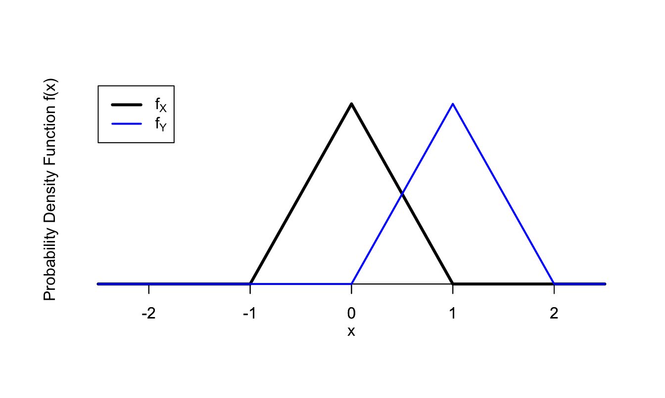

Figure 36.2: Example of a Shift Transformation

Theorem 36.2 (Scale Transformation) Let \(X\) be a continuous random variable with p.d.f. \(f_X\). The p.d.f. of \(Y = aX\), where \(a > 0\) is a constant, is \[\begin{equation} f_Y(y) = \frac{1}{a} f_X(\frac{y}{a}). \tag{36.2} \end{equation}\]

Proof. We can express the c.d.f. of \(Y\) in terms of the c.d.f. of \(X\): \[\begin{align*} F_Y(y) &= P(Y \leq y) \\ &= P(aX \leq y) \\ &= P(X \leq \frac{y}{a}) \\ &= F_X(\frac{y}{a}). \end{align*}\]

Taking the derivative (don’t forget the chain rule!), we see that the p.d.f. is \[ f_Y(y) = \frac{d}{dy} F_Y(y) = \frac{1}{a} f_X(\frac{y}{a}). \]

The figure below illustrates a hypothetical p.d.f. for a random variable \(X\) and the corresponding p.d.f. for the scaled random variable \(Y = 2X\). Notice that the p.d.f. is the same shape, just wider and shorter.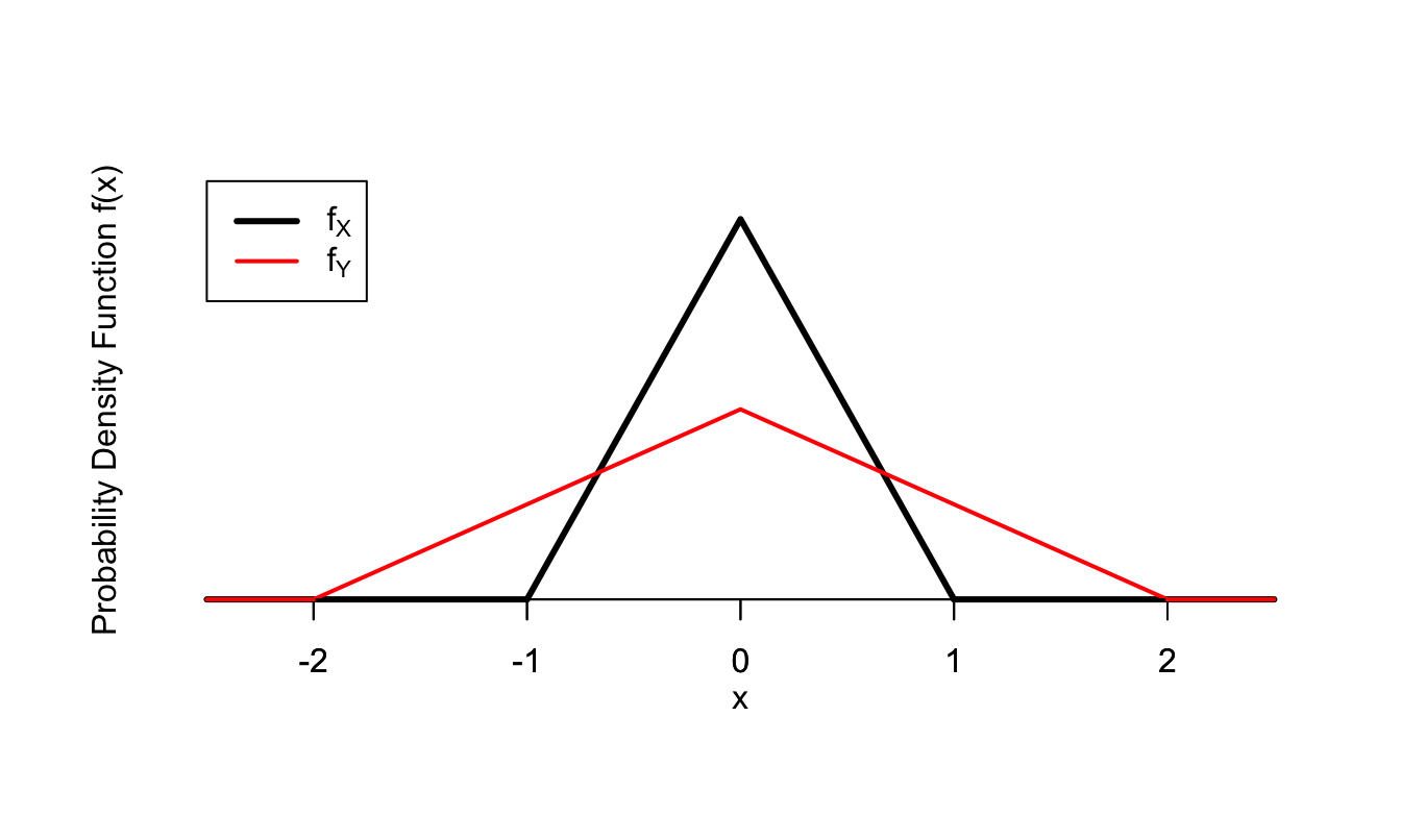

Figure 36.3: Example of a Scale Transformation

The factor of \(\frac{1}{a}\) on the inside in (36.2) is what makes the p.d.f. wider, and the factor of \(\frac{1}{a}\) on the outside is what makes it shorter. It is necessary to make the p.d.f. shorter if we make it wider, since the total area under a p.d.f. must always be 1.

Essential Practice

1. You inflate a spherical balloon in a single breath. If the volume of air you exhale in a single breath (in cubic inches) is \(\text{Uniform}(a=36\pi, b=288\pi)\) random variable, what is the p.d.f. of the radius of the balloon (in inches)?

2. The lifetime of a lightbulb (in hours) follows an \(\text{Exponential}(\lambda=\frac{1}{1200})\) distribution. Find the p.d.f. of the lifetime of the lightbulb in days (assuming the lightbulb is on 24 hours per day).

3. A lighthouse on a shore is shining light toward the ocean at a random angle \(U\) (measured in radians), where \(U\) follows a \(\text{Uniform}(a=-\frac{\pi}{2}, b=\frac{\pi}{2})\) distribution.

   Consider a line which is parallel to the shore and 1 mile away from the shore, as illustrated below. An angle of 0 would mean the ray of light is perpendicular to the shore, while an angle of \(\pi/2\) would mean the ray is along the shore, shining to the right from the perspective of the figure.

   

   Let \(X\) be the point that the light hits on the line, where the line’s origin is the point on the line that is closest to the lighthouse. Find the p.d.f. of \(X\).

   (Hint: Use trigonometry to write \(X\) as a function of \(U\).)

Additional Practice

1. The radius of a circle (in inches) is chosen from an \(\text{Exponential}(\lambda=1.5)\) distribution. Find the p.d.f. of the area of the circle.