Lesson 19 Marginal Distributions

Motivating Example

In Lesson 18, we found the joint distribution of $X$, the number of bets that Xavier wins, and $Y$, the number of bets that Yolanda wins. If all we have is the joint distribution of $X$ and $Y$, can we recover the distribution of $X$ alone?

Theory

Recall from Lesson 10 that the p.m.f. of $X$ is defined to be $P(X = x)$ as a function of $x$. To calculate a probaebility from a joint p.m.f., we sum over the relevant outcomes. In this case, we need to sum the joint p.m.f. over all the possible values of $y$ for the given $x$: \[\begin{equation} P(X = x) = \sum_y f(x, y). \tag{19.1} \end{equation}\]

If the joint p.m.f. is written out in table form, then (19.2) corresponds to the column sums of the table, as illustrated in Figure 19.1.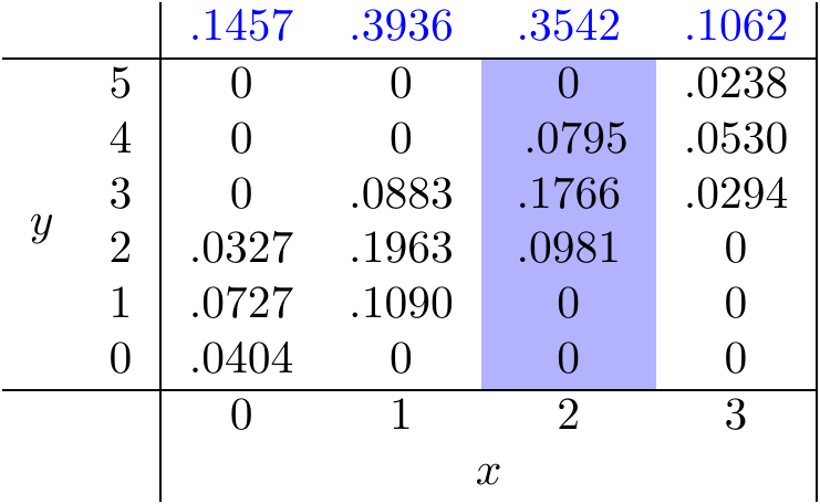

Figure 19.1: Calculating the Marginal Distribution of $X$

Notice how natural it was to write the column totals in the margins of the table in Figure 19.1. For this reason, this collection of probabilities has come to be known as the marginal distribution of $X$.

Definition 19.1 (Marginal Distribution) The marginal p.m.f. of $X$ refers to the p.m.f. of $X$ when it is calculated from the joint p.m.f. of $X$ and $Y$. Specifically, the marginal p.m.f. $f_X$ can be calculated from the joint p.m.f. $f$ as follows: \[\begin{equation} f_X(x) \overset{\text{def}}{=} P(X=x) = \sum_y f(x, y). \tag{19.2} \end{equation}\] Notice that we use subscripts in $f_X$ to distinguish this function from the joint distribution $f$ and, later, the marginal distribution of $Y$.

There is also a marginal distribution of $Y$. As you might guess, the marginal p.m.f. is symbolized $f_Y$ and is calculated by summing over all the possible values of $X$: \[\begin{equation} f_Y(y) \overset{\text{def}}{=} P(Y=y) = \sum_x f(x, y). \tag{19.3} \end{equation}\] On a table, the marginal distribution of $Y$ corresponds to the row sums of the table, as illustrated in Figure 19.2.

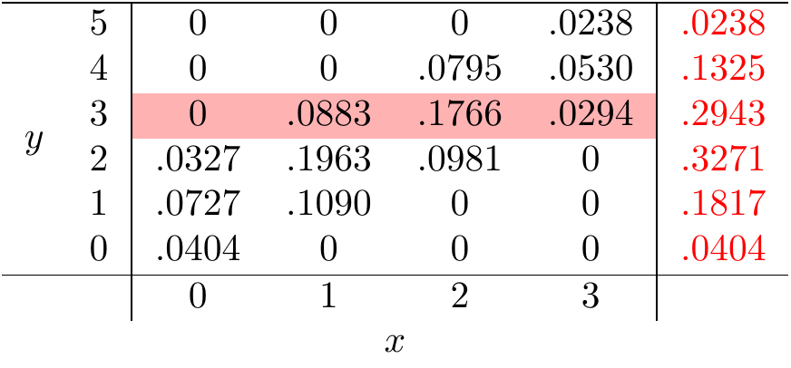
Figure 19.2: Calculating the Marginal Distribution of $Y$

Remember that we know the distribution of $Y$. It is $\text{Binomial}(n=5, p=18/38)$. You should verify that the marginal distribution we calculated in 19.2 matches that of a $\text{Binomial}(n=5, p=18/38)$ distribution.

Theorem 19.1 (Joint Distribution of Independent Random Variables) If $X$ and $Y$ are independent, then \[\begin{equation} f(x, y) = f_X(x) \cdot f_Y(y) \end{equation}\] for all values $x$ and $y$. But only if $X$ and $Y$ are independent!

Proof. In Lesson 18, we saw that the joint distribution is defined to be \[ f(x, y) = P(X = x \text{ and } Y=y). \] If $X$ and $Y$ are independent, then we can multiply the probabilities, by Theorem 7.1: \[ P(X=x) \cdot P(Y=y). \] But $P(X=x)$ is just the marginal distribution of $X$ and $P(Y=y)$ the marginal distribution of $Y$. So this is equal to: \[ f_X(x) \cdot f_Y(y) \]

Let’s calculate another marginal distribution—this time from the formula representation of the joint p.m.f.

Example 19.1 (Marginal Number of Chicks) In Example 18.3, we found that the joint distribution of the number of eggs $N$ and the number of chicks $X$ was \[\begin{equation} f(n, x) = \begin{cases} e^{-\mu} \frac{(\mu p)^x}{x!} \frac{(\mu (1-p))^{n-x}}{(n-x)!} & 0 \leq x \leq n < \infty \\ 0 & \text{otherwise} \end{cases}. \tag{19.4} \end{equation}\] What is the marginal distribution of the number of chicks, $X$?

Solution. By (19.2), we need to sum the joint p.m.f. $f(n, x)$ over all the possible values of $N$. In (19.4), we see that the joint p.m.f. is $0$ unless $n \geq x$. So we sum the complicated expression in (19.4) for all $n$ from $x$ to $\infty$. \[\begin{align*} f_X(x) &= \sum_n f(n, x) \\ &= \sum_{n=x}^\infty e^{-\mu} \frac{(\mu p)^x}{x!} \frac{(\mu (1-p))^{n-x}}{(n-x)!} \\ &= e^{-\mu} \frac{(\mu p)^x}{x!} \sum_{n=x}^\infty \frac{(\mu (1-p))^{n-x}}{(n-x)!} & \text{(pull out terms not depending on $n$)} \\ &= e^{-\mu} \frac{(\mu p)^x}{x!} \sum_{m=0}^\infty \frac{\nu^m}{m!} & (m=n-x, \nu=\mu(1-p)) \\ &= e^{-\mu} \frac{(\mu p)^x}{x!} e^{\nu} \underbrace{\sum_{m=0}^\infty e^{-\nu} \frac{\nu^m}{m!}}_{\text{sum of Poisson$(\nu)$ p.m.f.} = 1} & \text{(multiply by $e^{\nu} e^{-\nu} = 1$)} \\ &= e^{-\mu + \mu(1-p)} \frac{(\mu p)^x}{x!} & (e^{-\mu + \nu}, \nu=\mu(1-p)) \\ &= e^{-\mu p} \frac{(\mu p)^x}{x!}. \end{align*}\] This formula is valid for $x=0, 1, 2, \ldots$. We recognize this as the p.m.f. of a $\text{Poisson}(\mu p)$ distribution.

Essential Practice

Let $X$ be the number of times a certain numerical control machine will malfunction on a given day. Let $Y$ be the number of times a technician is called on an emergency call. Their joint p.m.f. is given by \[ \begin{array}{rr|cccc} & 5 & 0 & .20 & .10 \\ y & 3 & .05 & .10 & .35 \\ & 1 & .05 & .05 & .10 \\ \hline & & 1 & 2 & 3\\ & & & x \end{array}. \]
1. Calculate the marginal distribution of $X$.
2. Calculate the marginal distribution of $Y$.
3. Are $X$ and $Y$ independent? How do you know?
Use the joint p.m.f. of the smaller and the larger of two dice rolls that you calculated in Lesson 18 to find the p.m.f. of the larger number. Use this p.m.f. to solve the “last banana” problem from Lesson 7.
Suppose two random variables $X$ and $Y$ both have marginal $\text{Binomial}(n=3, p=0.5)$ distributions. In this exercise, you will see that there are many joint distributions that could have those marginal distributions.
1. What is the joint p.m.f. if $X$ and $Y$ are independent?
2. Can you find at least 2 more joint p.m.f.s with the same marginal distributions? (Hint: What happens if you define $X$ and $Y$ based on just 3 tosses of a coin? What about 4 tosses of a coin?)

Additional Exercises

Two tickets are drawn without replacement from a box with $N_1$ $\fbox{1}$s and $N_0$ $\fbox{0}$s. Let $X$ be the number of $\fbox{1}$s on the first draw and $Y$ be the number of $\fbox{1}$s on the second draw. It is clear that the first draw has a $\frac{N_1}{N}$ probability of being a $\fbox{1}$. But what about the second draw?

In Lesson 18, you found the joint distribution of $X$ and $Y$. Use this joint p.m.f. to show that the probability that the second draw is a $\fbox{1}$ is $\frac{N_1}{N}$.