Lesson 48 Examples of Random Processes

In this lesson, we cover a few more examples of random processes.

Example 48.1 (Random Amplitude Process) Let \(A\) be a random variable. Let \(f\) be a constant. Then the continuous-time process \[ X(t) = A\cos(2\pi f t) \] is called a random amplitude process.

Note that once the value of \(A\) is simulated, the random process \(\{ X(t) \}\) is completely specified for all times \(t\).

Shown below are 30 realizations of the random amplitude process, where \(A\) is \(\text{Binomial}(n=5, p=0.5)\).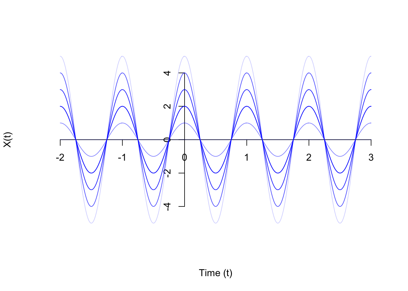

Here is a video that animates the random amplitude process.

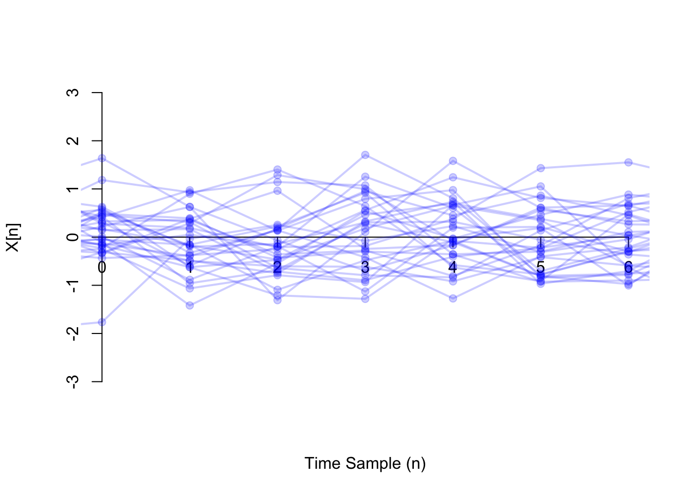
Example 48.2 (Moving Average Process) Let \(\{ Z[n] \}\) be a white noise process. Then, a moving average process (of order 1) \(\{ X[n] \}\) is a discrete-time process defined by \[\begin{equation} X[n] = b_0 Z[n] + b_1 Z[n-1]. \tag{48.1} \end{equation}\]

Below, we show one realization of a white noise process \(\{ Z[n] \}\) (in orange), along with the corresponding moving average process \[ X[n] = 0.5 Z[n] + 0.5 Z[n-1]. \] Notice that the moving average process is just the average of successive values of the white noise process. As a result, the moving average process is “smoother” than the white noise process.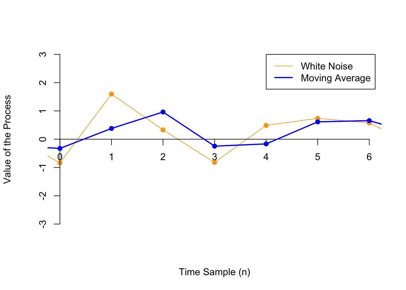

Now, we show 30 realizations of the same moving average process. Superficially, this might look like the white noise of Example 47.2, but if you look closely, you will see that each individual function fluctuates less.