Lesson 45 Sums of Continuous Random Variables
Theory
Let \(X\) and \(Y\) be independent continuous random variables. What is the distribution of their sum— that is, the random variable \(T = X + Y\)? In Lesson 21, we saw that for discrete random variables, we convolve their p.m.f.s. In this lesson, we learn the analog of this result for continuous random variables.
Comparing this with Theorem 21.1, we see once again that the only difference between the discrete case and the continuous case is that sums are replaced by integrals and p.m.f.s by p.d.f.s.
Proof. Since \(T\) is a continuous random variable, we find its c.d.f. and take derivatives. Let \(f\) denote the joint distribution of \(X\) and \(Y\). We know that \(f(x, y)\) factors as \(f_X(x)\cdot f_Y(y)\) by Theorem 42.1, since \(X\) and \(Y\) are independent. \[\begin{align*} F_T(t) = P(T \leq t) &= P(X + Y \leq t) \\ &= \int_{-\infty}^\infty \int_{-\infty}^{t-x} f(x, y) \,dy\,dx \\ &= \int_{-\infty}^\infty \int_{-\infty}^{t-x} f_X(x) \cdot f_Y(y) \,dy\,dx \\ &= \int_{-\infty}^\infty f_X(x) \int_{-\infty}^{t-x} f_Y(y) \,dy\,dx \\ &= \int_{-\infty}^\infty f_X(x) F_Y(t-x) \,dx, \end{align*}\] where in the last step, we used the definition of the c.d.f. of \(Y\). (We are calculating the area under the p.d.f. of \(Y\) up to \(t-x\).)
Now, we take the derivative with respect to \(t\). The integral behaves like a sum, so we can move the derivative inside the integral sign. Also, \(f_X(x)\) is a constant with respect to \(t\). \[\begin{align*} \frac{d}{dt} F_T(t) &= \int_{-\infty}^\infty f_X(x) \frac{d}{dt} F_Y(t-x) \,dx \\ &= \int_{-\infty}^\infty f_X(x) f_Y(t-x) \,dx, \end{align*}\] as we wanted to show.Example 45.1 (Sum of Independent Uniforms) Let \(X\) and \(Y\) be independent \(\text{Uniform}(a=0, b=1)\) random variables. What is the p.d.f. of \(T = X + Y\)?
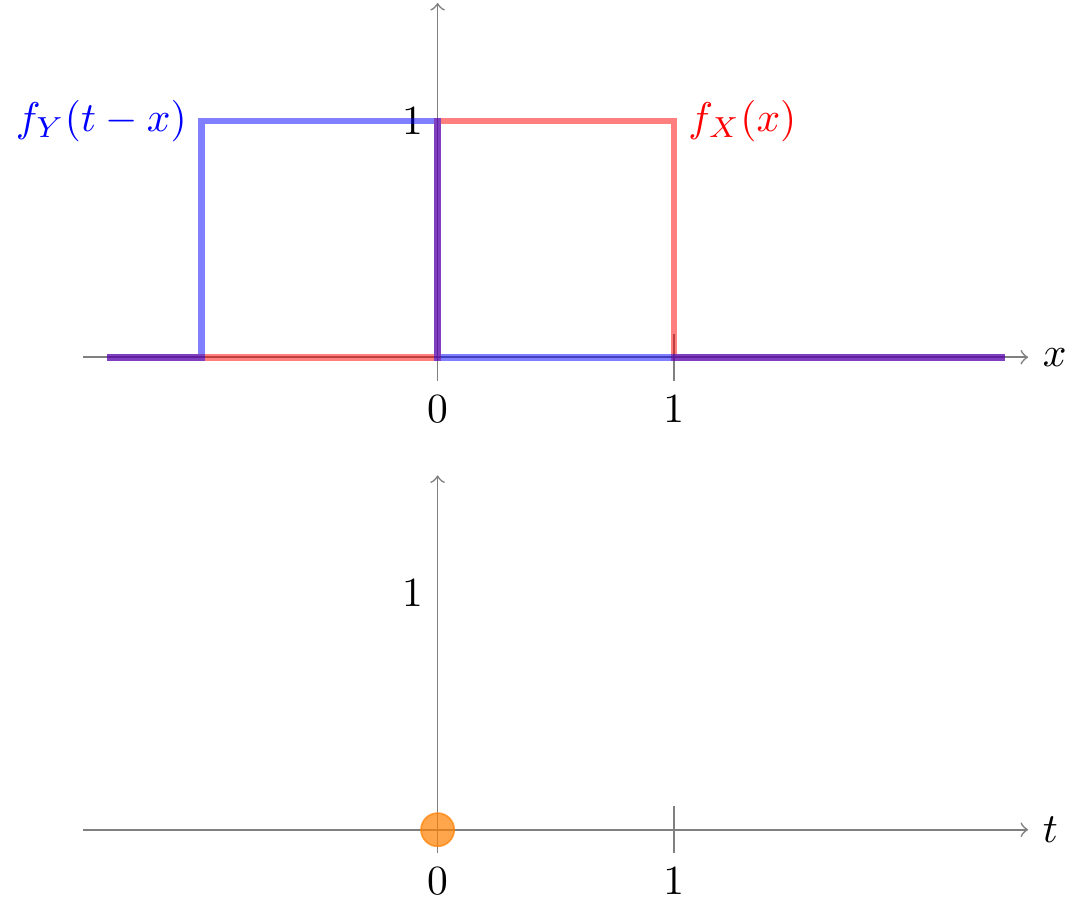
We have to convolve the p.d.f. of \(X\) with the p.d.f. of \(Y\). The p.d.f.s of both \(X\) and \(Y\) are \[ f(x) = \begin{cases} 1 & 0 < x < 1 \\ 0 & \text{otherwise} \end{cases}. \] This is a rectangle function.
To calculate the convolution, we first flip \(f_Y\) about the \(y\)-axis. We then integrate the product of \(f_X\) and the flipped version of \(f_Y\) to obtain the convolution at \(t=0\). In this case, the two functions are never both non-zero, so the integral is 0.
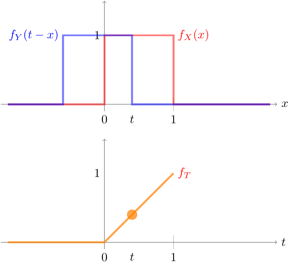
Now, to get the convolution at \(t\), we shift the flipped version of \(f_Y\) to the right by \(t\). This is why the convolution operation is often called “flip and shift”. To see why, consider the formula when we flip and shift \(f_Y\): \[\begin{align*} \text{FLIP}[f_Y](x) &= f_Y(-x) \\ \text{SHIFT}_t[\text{FLIP}[f_Y]](x) &= \text{FLIP}[f_Y](x - t) \\ &= f_Y(-(x - t)) \\ &= f_Y(t - x). \\ \end{align*}\] This is exactly the term that we multiply by \(f_X(x)\) in the convolution formula (45.1) before integrating.
For the uniform distribution, there are two cases. If we shift (the flipped version of \(f_Y\)) by some amount \(0 < t < 1\), then the supports of the two distributions overlap between \(0\) and \(t\), so the result of the convolution is \[ f_T(t) = \int_0^t 1 \cdot 1\,dx = t. \]
On the other hand, if we shift by some amount \(1 < t < 2\), then the supports of the two distributions overlap between \(t-1\) and \(1\), so the result of the convolution is \[ f_T(t) = \int_{t-1}^1 1 \cdot 1\,dx = 2 - t. \]
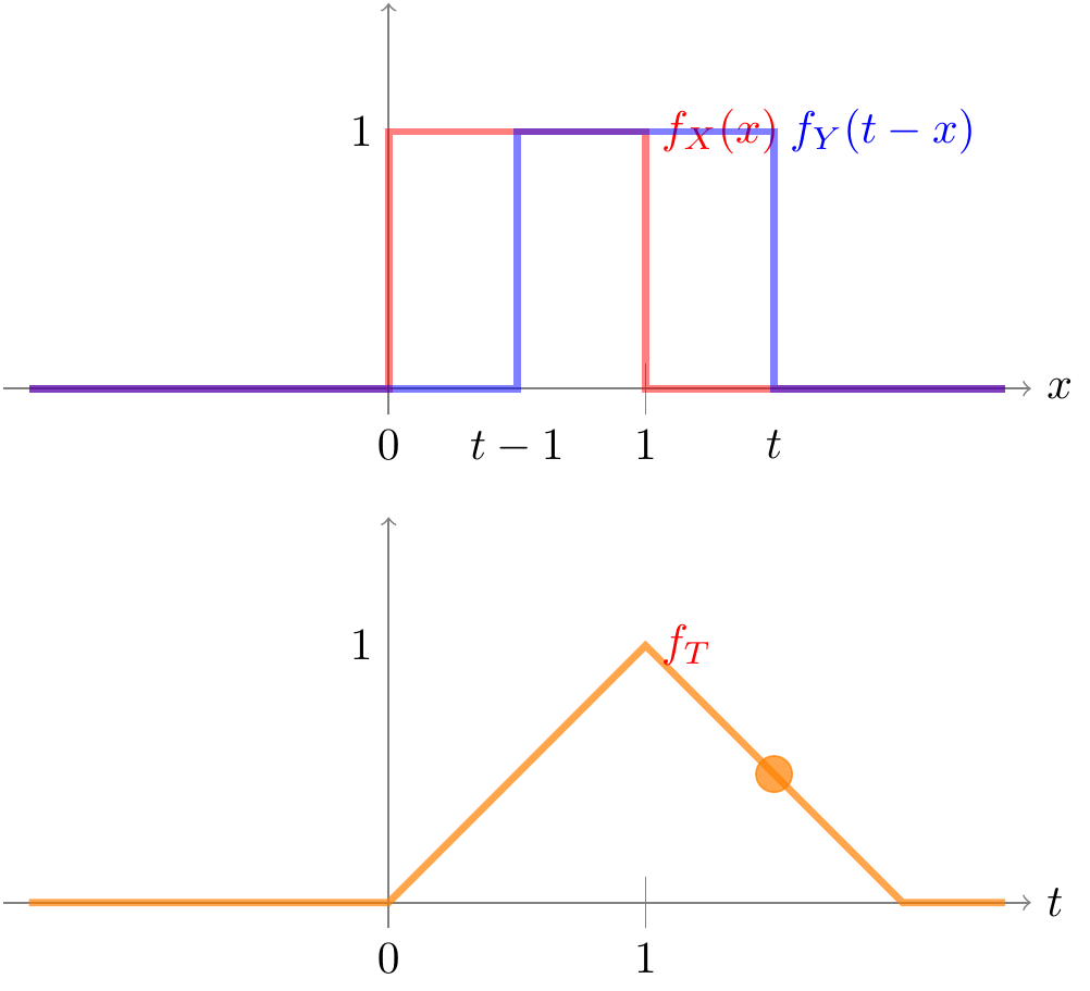
Putting it all together, the formula for the p.d.f. is given by \[ f_T(t) = \begin{cases} t & 0 < t \leq 1 \\ 2 - t & 1 < t < 2 \\ 0 & \text{otherwise} \end{cases}. \] This is sometimes known as the triangular distribution, for obvious reasons.
Example 45.2 (Distribution of the Arrival Times) In Examples 43.3 and 44.3, we derived the expectation and standard deviation of \(S_r\), the \(r\)th arrival time by writing \(S_r\) as a sum of the \(\text{Exponential}(\lambda=0.8)\) interarrival times: \[ S_r = T_1 + T_2 + \ldots + T_r. \] In this example, we investigate the distribution of \(S_r\).
We start with the case \(r=2\). Since \(S_2\) is the sum of \(T_1\) and \(T_2\), two independent exponential random variables, we can use Theorem 45.1 to derive its p.d.f.
We convolve the \(\text{Exponential}(\lambda=0.8)\) p.d.f. with itself, since \(T_1\) and \(T_2\) have the same distribution. Plugging the p.d.f.s into (45.1), we obtain: \[ f_{S_2}(t) = \int_{?}^? 0.8 e^{-0.8 x} \cdot 0.8 e^{-0.8 (t - x)}\,dx, \] where the limits of integration are TBD.
To determine the limits of integration, there are several ways to think about it:
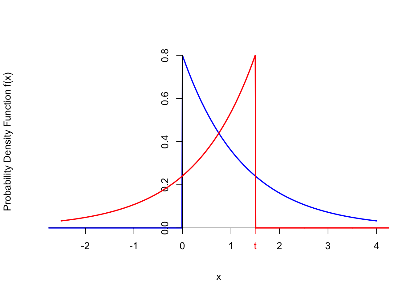
- Remember that the support of the exponential distribution is on the positive numbers. Therefore, the integrand will be 0, unless both \(x\) and \((t-x)\) are positive. This means that the limits of integration must be from \(0\) to \(t\).
- \(f_{S_2}(t)\) captures how likely it is for the second arrival to happen “near” \(t\) seconds. If \(x > t\), then the first arrival happened after \(t\) seconds, so the second arrival could not have happened near \(t\) seconds.
- If we flip and shift one of the exponential distributions, then the supports of the two functions will only overlap between \(0\) and \(t\), as illustrated in the graph below.
Now that we have the limits of integration, we obtain the following formula for the p.d.f. for \(t > 0\). \[\begin{align*} f_{S_2}(t) &= \int_0^t 0.8 e^{-0.8 x} \cdot 0.8 e^{-0.8 (t - x)}\,dx \\ &=\int_0^t (0.8)^2 e^{-0.8 (x + (t - x))}\,dx \\ &= (0.8)^2 e^{-0.8 t} \int_0^t 1\,dx \\ &= (0.8)^2 t e^{-0.8 t}; t > 0 \end{align*}\]
This p.d.f. is graphed in red, along with the exponential p.d.f. of the interarrival times in gray.
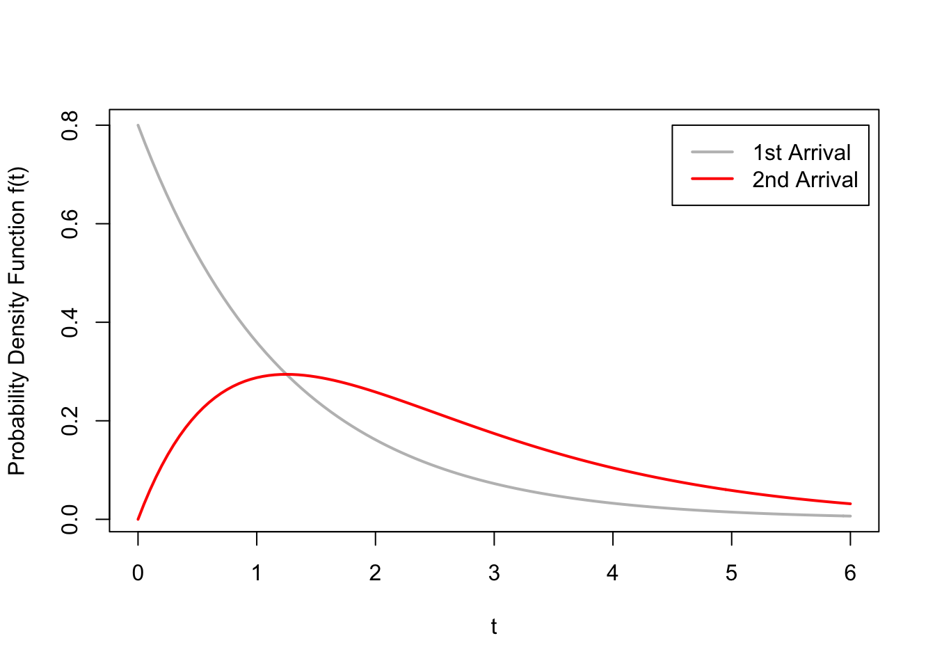 From the figure above, we see that the second arrival tends to happen later than the first arrival,
which makes intuitive sense. The p.d.f. also seems to be centered around \(2 / 0.8 = 2.5\),
which is the expected value we calculated in Example 43.3.
From the figure above, we see that the second arrival tends to happen later than the first arrival,
which makes intuitive sense. The p.d.f. also seems to be centered around \(2 / 0.8 = 2.5\),
which is the expected value we calculated in Example 43.3.
What about when \(r=3\)? The time of third arrival is the sum of the time of the second arrival, \(S_2\), and the
time between the second and third arrivals, \(T_3\). Therefore, to obtain the p.d.f. of \(S_3\), we convolve
the p.d.f. of \(S_2\) we derived above with the \(\text{Exponential}(\lambda=0.8)\)
p.d.f. The right limits of integration are \(0\) to \(t\), by the same argument as above.
\[\begin{align*}
f_{S_3}(t) &= \int_0^t (0.8)^2 x e^{-0.8 x} \cdot 0.8 e^{-0.8 (t - x)}\,dx \\
&=\int_0^t (0.8)^3 x e^{-0.8 (x + (t - x))}\,dx \\
&= (0.8)^3 e^{-0.8 t} \int_0^t x\,dx \\
&= \frac{(0.8)^3}{2} t^2 e^{-0.8 t}; t > 0
\end{align*}\]
This p.d.f. is graphed in blue below.
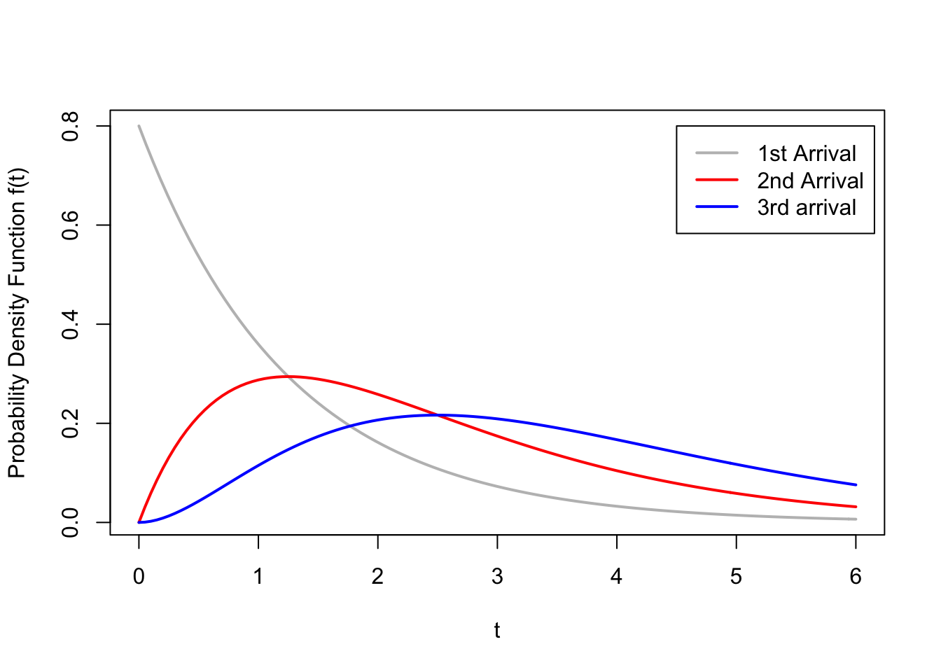
In general, we can continue in this way to obtain the following formula for the p.d.f. of the \(r\)th arrival time in this Poisson process. \[\begin{equation} f_{S_r}(t) = \frac{(0.8)^r}{(r-1)!} t^{r-1} e^{-0.8 t}; t > 0. \tag{45.2} \end{equation}\] This family of distributions is known as the gamma distribution, with parameters \(r\) and \(\lambda =0.8\).
Essential Practice
In this exercise, you will investigate the distribution of \(S_n = U_1 + U_2 + \ldots + U_n\), where \(U_i\) are i.i.d. \(\text{Uniform}(a=0, b=1)\) random variables. You already calculated \(E[S_n]\) and \(\text{SD}[S_n]\) in Lesson 44. Now, you will calculate its distribution.
Find the p.d.f. of \(S_3 = U_1 + U_2 + U_3\) and sketch its graph. Check that this p.d.f. agrees with the value of \(E[S_3]\) and \(\text{SD}[S_3]\) that you calculated earlier.
(Hint 1: We already worked out the distribution of \(U_1 + U_2\) in Example 45.1. Do another convolution.)
(Hint 2: You should end up with a p.d.f. with 4 cases: \(f_{S_3}(t) = \begin{cases} ... & 0 < t \leq 1 \\ ... & 1 < t \leq 2 \\ ... & 2 < t < 3 \\ 0 & \text{otherwise} \end{cases}\).)
Find the p.d.f. of \(S_4 = U_1 + U_2 + U_3 + U_4\) and sketch its graph. Check that this p.d.f. agrees with the value of \(E[S_4]\) and \(\text{SD}[S_4]\) that you calculated earlier.
(Hint: I think the easiest way to do this is to convolve another uniform p.d.f. with the p.d.f. you got in part a. However, you could also do this by convolving two triangle functions together. You should get the same answer either way.)
Neither \(S_3\) nor \(S_4\) are named distributions. However, if you sketch their p.d.f.s, they should remind you of one of the named distributions we learned. Which one?
Let \(X\) and \(Y\) be independent standard normal—that is, \(\text{Normal}(\mu=0, \sigma=1)\)—random variables. Let \(T = X + Y\). You should quickly be able to determine \(E[T]\) and \(\text{Var}[T]\). But what is the distribution of \(T\)? Use convolution to answer this question.
(I’m happy if you can just set up the integral and plug it into Wolfram Alpha. If you really want to solve it by hand, try “completing the square” in the exponent so that you end up with something that looks like a normal p.d.f., which you know must integrate to 1.)
(This exercise is an application of the result that you found in the previous exercise. It is otherwise unrelated to this lesson.) Let \(X_1\), \(X_2\), and \(X_3\) represent the times (in minutes) necessary to perform three successive repair tasks at a service facility. They are independent, normal random variables with expected values 45, 50, and 75 and variances 10, 12, and 14, respectively. What is the probability that the service facility is able to finish all three tasks within 3 hours (that is, 180 minutes)?
(Hint: Use the previous exercise to identify the distribution of \(T = X_1 + X_2 + X_3\). It is one of the named distributions we learned. Once you identify the distribution and its parameters, you can calculate the probability in the usual way. You should not need to do any convolutions to answer this question.)