Lesson 58 LTI Filters in the Frequency Domain

Motivation

In Lesson 57, we studied what LTI filters do to stationary signals in the time domain. However, it is usually easier to analyze and understand LTI filters in the frequency domain, as we explore in this lesson.

Theory

Theorem 58.1 (Filter Theorem) Let \(\{ X(t) \}\) be a stationary random process with power spectral density \(S_X(f)\). If \(\{ X(t) \}\) is passed into a linear time-invariant filter with impulse response \(h(t)\), then the output process \(\{ Y(t) \}\) has power spectral density \[\begin{equation} S_Y(f) = |H(f)|^2 \cdot S_X(f), \tag{58.1} \end{equation}\] where \(H(f)\) is the frequency response of the filter (i.e., the Fourier transform of the impulse response).

Show/Hide Proof

Proof. Theorem 57.2 provides the mean and autocovariance functions of \(\{ Y(t) \}\). We can use these to obtain the autocorrelation function of \(\{ Y(t) \}\): \[\begin{align*} R_Y(\tau) &= C_Y(\tau) + \mu_Y^2 \\ &= (h(-t) * h * C_X)(\tau) + \left(\mu_X \int_{-\infty}^\infty h(t)\,dt\right)^2 \\ &= (h(-t) * h * C_X)(\tau) + (h(-t) * h * \mu_X^2) \\ &= (h(-t) * h * R_X)(\tau). \end{align*}\] The second-to-last equality follows from the fact that the convolution of any function with a constant function (\(\mu_X^2\)) is itself a constant function. So \(h * \mu_X^2\) is the constant \(\int_{-\infty}^\infty h(t)\,dt \mu_X^2\), and convolving this constant function with \(h(-t)\) gives another factor of \(\int_{-\infty}^\infty h(t)\,dt\).

Now, we know that \(S_Y\), the power spectral density of \(\{ Y(t) \}\), is just the Fourier transform of the autocorrelation function \(R_Y\). Combining the representation of \(R_Y\) above with the Fourier properties from Appendix D.3, we obtain: \[\begin{align*} S_Y(f) &= \mathscr{F}[R_Y](f) \\ &= \mathscr{F}[h(-t) * h * R_X](f) \\ &= \mathscr{F}[h(-t)](f) \cdot \mathscr{F}[h](f) \cdot \mathscr{F}[R_X](f) & \text{(convolution property)} \\ &= H(-f) \cdot H(f) \cdot S_Y(f) & \text{(definitions of $H$ and $S_Y$, reversal property)} \\ &= H^*(f) \cdot H(f) \cdot S_X(f) & \text{($h$ is real, so $H$ is conjugate symmetric)} \\ &= |H(f)|^2 \cdot S_X(f), \end{align*}\] as we wanted to show.

Example 58.1 (White Noise) Consider the white noise process \(\{ Z[n] \}\) defined in Example 47.2, which consists of i.i.d. random variables with mean \(\mu = E[Z[n]]\) and variance \(\sigma^2 \overset{\text{def}}{=} \text{Var}[Z[n]]\).

We showed in Example 56.1 that its PSD is \[ S_Z(f) = \sigma^2 + \mu^2 \delta(f). \]

Let’s pass \(\{ Z[n] \}\) through a filter with impulse response \[ h[n] = (-0.4)^n u[n]. \] What is the PSD of the output \(\{ Y[n] \}\)?

Solution. By the Filter Theorem (Theorem 58.1), we know that \[ S_Y(f) = |H(f)|^2 \cdot S_Z(f). \] So all we need to do is find \(|H(f)|^2\).

By Table D.2, the frequency response of the filter is \[ H(f) = \frac{1}{1 + 0.4e^{-j2\pi f}} \] so \[\begin{align*} |H(f)|^2 &= H(f) \cdot H^*(f) \\ &= \frac{1}{1 + 0.4e^{-j2\pi f}} \cdot \frac{1}{1 + 0.4e^{j2\pi f}} \\ &= \frac{1}{1 + 0.4 (e^{j2\pi f} + e^{-j2\pi f}) + (0.4)^2} \\ &= \frac{1}{1.16 + 0.8\cos(2\pi f)}. \end{align*}\]

Now, \(S_Y(f)\) is just the product of this and \(S_Z(f)\). \[\begin{align*} S_Y(f) &= \frac{1}{1.16 + 0.8\cos(2\pi f)} \cdot (\sigma^2 + \mu^2 \delta(f)) \\ &= \frac{\sigma^2}{1.16 + 0.8\cos(2\pi f)} + \frac{\mu^2}{1.16 + 0.8\cos(2\pi \cdot 0)} \delta(f). \end{align*}\] The last equality follows from the fact that \(\delta(f) = 0\) everywhere except \(f=0\), so we can substitute \(f=0\) into the coefficient.

The graphs below show:

• the PSD of the input \(S_Z(f)\) (in red),
• the squared magnitude of the frequency response \(|H(f)|^2\) (in blue), and
• the PSD of the output \(S_Y(f)\) (in orange),

for \(\mu=-1.5\) and \(\sigma^2 = 1.7\). Notice that the filter \(h\) is a highpass filter, passing high frequencies (i.e., near the Nyquist limit of 0.5) and attenuating low frequencies.

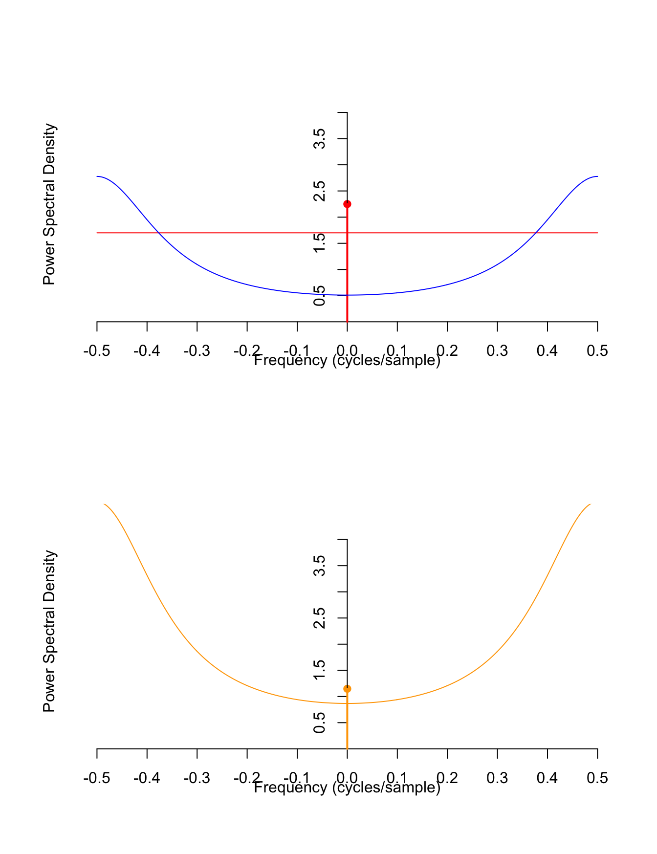
We can calculate the expected power in the output signal \(\{ Y[n] \}\) by integrating the PSD over “all” frequencies. (This is the easiest way, since the autocorrelation function \(R_Y[k]\) is not available.) Because this is a discrete-time signal, we only integrate over frequencies below the Nyquist limit, \(|f| < 0.5\). \[\begin{align*} \int_{-0.5}^{0.5} S_Y(f)\,df &= \int_{-0.5}^{0.5} \frac{\sigma^2}{1.16 + 0.8\cos(2\pi f)} \,df + \int_{-0.5}^{0.5} \frac{\mu^2}{1.96} \delta(f)\,df \\ &\approx 1.1905 \sigma^2 + \frac{\mu^2}{1.96}. \end{align*}\]

Example 58.2 Consider the process \(\{X(t)\}\) from Example 53.5 with autocorrelation function \[ R_X(\tau) = 5 e^{-\tau^2 / 3} + 4. \] We showed in Example 56.2 that its power spectral density is \[\begin{align*} S_X(f) &= 5 \sqrt{\frac{\pi}{3}} e^{-\pi^2 f^2 / 3} + 4 \delta(f) \end{align*}\] Now, suppose we pass \(\{ X(t) \}\) through an LTI filter with impulse response \[ h(t) = 1.8\text{sinc}(1.2t). \] Using the table in Appendix D.1, along with the scaling property, we see that the frequency response is \[ H(f) = 1.8\frac{1}{1.2} \text{rect}(\frac{f}{1.2}) = \begin{cases} 1.5 & |f| < 0.6 \\ 0 & \text{otherwise} \end{cases}. \] The filter \(h\) is an ideal lowpass filter because it perfectly passes frequencies below \(0.6\) Hz and perfectly rejects frequencies above \(0.6\) Hz. It is “ideal” because the impulse response \(h(t)\) is not implementable in practice. (The \(\text{sinc}\) function extends infinitely far into the past and into the future.)

Now, we have to calculate the squared magnitude of the impulse response for the filter theorem: \[ |H(f)|^2 = \begin{cases} 1.5^2 & |f| < 0.6 \\ 0 & \text{otherwise} \end{cases}. \]

\(S_X(f)\) and \(|H(f)|^2\) are graphed below.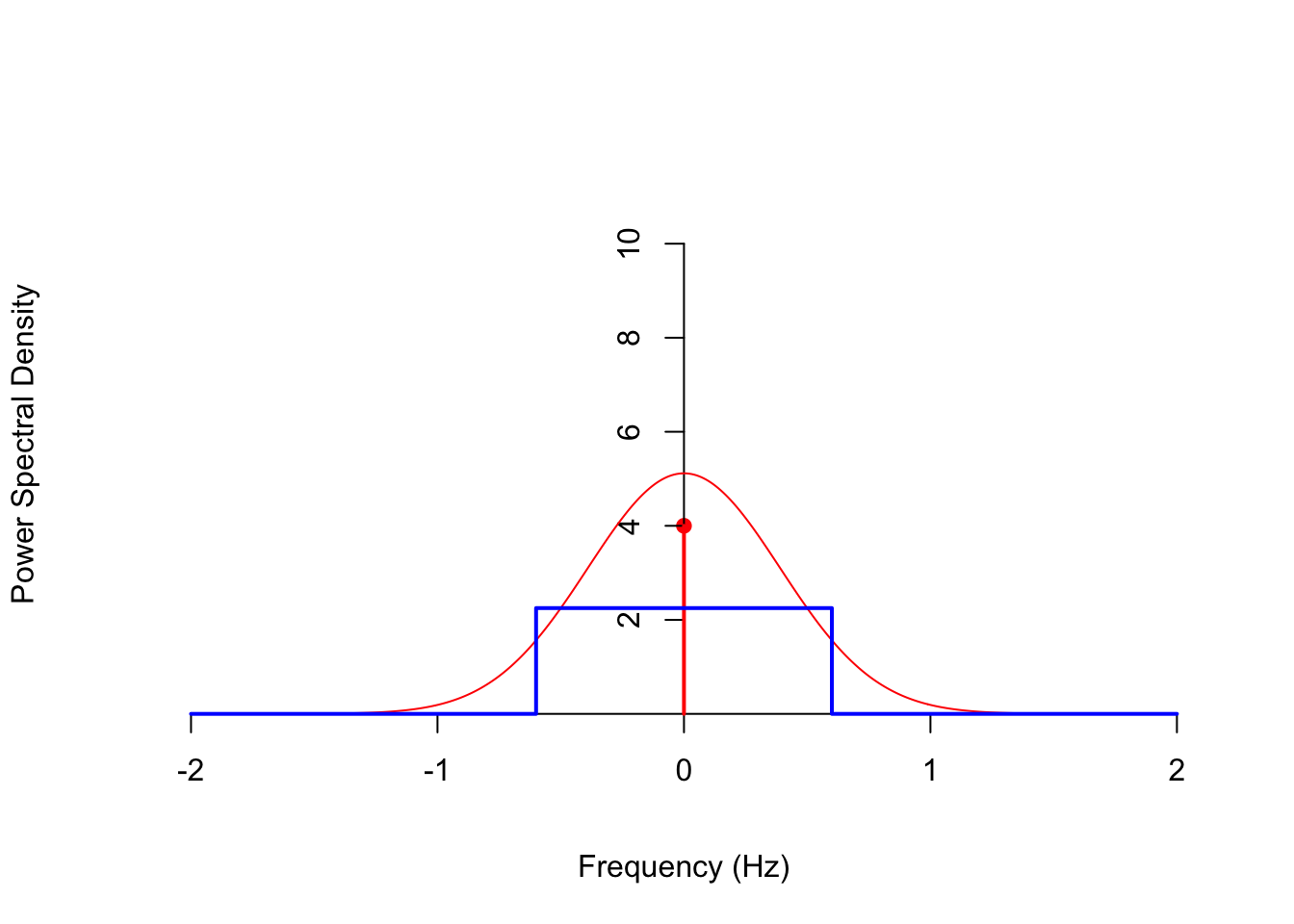

By the Filter Theorem (Theorem 58.1), the PSD of the output is \[ S_Y(f) = |H(f)|^2 \cdot S_X(f) = \begin{cases} 1.5^2 \cdot 5 \sqrt{\frac{\pi}{3}} e^{-\pi^2 f^2 / 3} + 1.5^2 \cdot 4 \delta(f) & |f| < 0.6 \\ 0 & \text{otherwise} \end{cases} \] The formula for \(S_Y(f)\) is quite messy; it is easier to understand what is going on by just graphing the function.

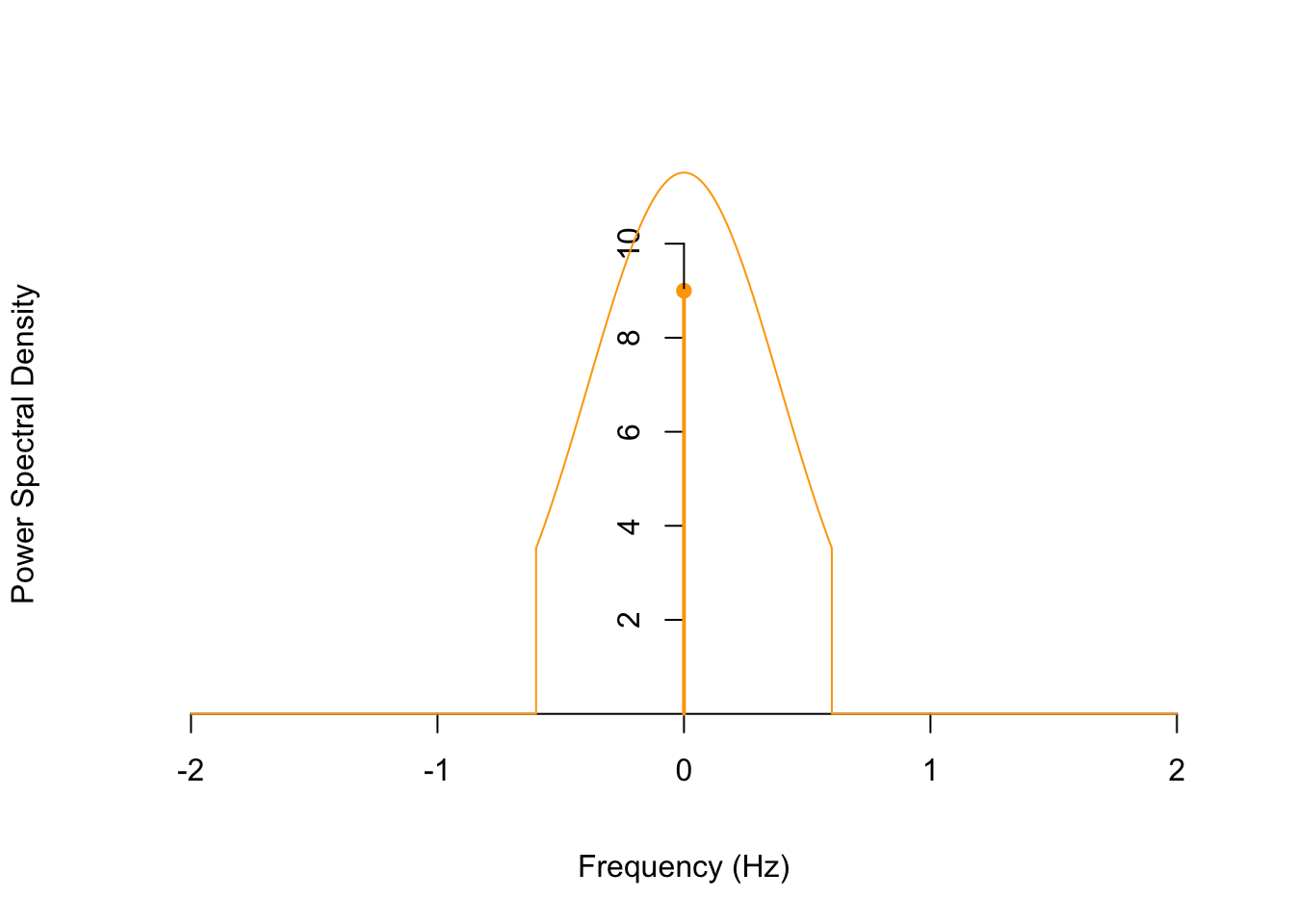
Frequencies below 0.6 Hz are passed (with a gain of \(1.5^2 = 2.25\)), while frequencies above 0.6 Hz are rejected.

The Filter Theorem allows us to prove a fact about power spectral densities that we have assumed in many of our calculations. Combined with Theorem 56.1, the next theorem justifies the name “power spectral density” for \(S_X(f)\).

Theorem 58.2 (Expected Power in a Frequency Band) The integral of the PSD \(S_X(f)\) over any frequency band \(a < |f| < b\) equals the expected power in that frequency band.

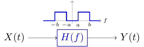
Proof. To measure the expected power in a signal \(\{ X(t) \}\) over the frequency band \(a < |f| < b\), we imagine passing \(\{ X(t) \}\) through the ideal bandpass filter \[ H(f) = \begin{cases} 1 & a < |f| < b \\ 0 & \text{otherwise} \end{cases}. \] The output signal \(\{ Y(t) \}\) is then just \(\{ X(t) \}\) with frequency content outside \(a < |f| < b\) removed.

Now, to obtain the expected power in \(\{ X(t) \}\) this frequency band, we can integrate the PSD of \(\{ Y(t) \}\) over all frequencies (by Theorem 56.1): \[ \text{Expected power between $a$ and $b$} = \int_{-\infty}^\infty S_Y(f)\,df. \] (This is for a continuous-time process. For a discrete-time process, the limits of the integral would be \(-0.5\) to \(0.5\).)

But by the Filter Theorem (Theorem 58.1), we have \[ \int_{-\infty}^\infty S_Y(f)\,df = \int_{-\infty}^\infty |H(f)|^2 S_X(f)\,df = \int_{a < |f| < b} S_X(f)\,df, \] since \(|H(f)|^2\) is 0 outside \(a < |f| < b\). This shows that we can obtain the expected power in ${X(t)} over any frequency band by integrating its PSD \(S_X(f)\) over the appropriate frequencies.

Essential Practice

For these questions, you may want to refer to the power spectral densities that you calculated in Lesson 56.

1. Radioactive particles hit a Geiger counter according to a Poisson process at a rate of \(\lambda=0.8\) particles per second. Let \(\{ N(t); t \geq 0 \}\) represent this Poisson process.

   Define the new process \(\{ D(t); t \geq 3 \}\) by \[ D(t) = N(t) - N(t - 3). \] This process represents the number of particles that hit the Geiger counter in the last 3 seconds.

   Suppose \(\{ D(t) \}\) is passed through an LTI filter with impulse response \[ h(t) = 3\text{sinc}(2t). \]

   What is the power spectral density of the output? What is the expected power in the output?

2. Consider the moving average process \(\{ X[n] \}\) of Example 48.2, defined by \[ X[n] = 0.5 Z[n] + 0.5 Z[n-1], \] where \(\{ Z[n] \}\) is a sequence of i.i.d. standard normal random variables.

   In Lesson 57, you expressed \(\{ X[n] \}\) as white noise passed through an LTI filter and calculated the impulse response of this filter. Use this impulse response and the PSD of white noise to calculate the PSD of this moving average process. Check that your answer agrees with the one you obtained in Lesson 56.

3. Let \(\{ X(t) \}\) be a continuous-time random process with mean function \(\mu_X(t) = -1\) and autocovariance function \(C_X(s, t) = 2e^{-|s - t|/3}\).

   If \(\{X(t)\}\) is passed through an LTI filter with impulse response \[ h(t) = \begin{cases} 4e^{-2t} & t \geq 0 \\ 0 & \text{otherwise} \end{cases}, \] what is the expected power in the output?