Lesson 56 Power Spectral Density
Motivation
In Lesson 55, we saw that the expected power of a stationary random signal \(\{ X(t) \}\) could be calculated by evaluating the autocorrelation function \(R_X(\tau)\) at a difference of \(\tau = 0\). But how is this expected power distributed across different frequencies? The answer also involves the autocorrelation function.
Theory
Definition 56.1 (Power Spectral Density) The power spectral density (or PSD, for short) \(S_X(f)\) of a stationary
random process \(\{ X(t) \}\) is the Fourier transform of the autocorrelation function
\(R_X(\tau)\). (Note: Because the process is stationary, the autocorrelation
only depends on the difference \(\tau = s - t\).)
That is, the autocorrelation function and the power spectral density are Fourier pairs. \[\begin{equation} R_X(\tau) \overset{\mathscr{F}}{\longleftrightarrow} S_X(f). \tag{56.1} \end{equation}\]
Because the autocorrelation function \(R_X(\tau)\) is symmetric and real-valued, its Fourier transform is guaranteed to also be symmetric and real-valued. See the Essential Practice exercise in Appendix C.The term “power spectral density” suggests that \(S_X(f)\) satisfies two properties:
- the integral of \(S_X(f)\) over all frequencies equals the expected power
- the integral of \(S_X(f)\) over any frequency band equals the expected power in that frequency band.
For now, we will only prove the first property, deferring the proof of the second property to Lesson 58.
Theorem 56.1 (Power Spectral Density and Expected Power) The integral of the PSD \(S_X(f)\) over “all” frequencies equals the expected power in \(\{ X(t) \}\).
For continuous-time processes, this result can be stated as: \[\begin{equation} \int_{-\infty}^\infty S_X(f)\,df = R_X(0) = E[X(t)^2]. \end{equation}\]
For discrete-time processes, this result can be stated as: \[\begin{equation} \int_{-0.5}^{0.5} S_X(f)\,df = R_X[0] = E[X[n]^2]. \end{equation}\]Proof. We will prove the result for continuous-time processes. The proof for discrete-time processes is similar.
By the “DC offset” property of Fourier transforms (Appendix D.3), the total integral of a signal in the time domain equals the value of the signal at 0 in the frequency domain, and vice versa. To prove this, observe that \[ G(0) \overset{\text{def}}{=} \int_{-\infty}^\infty g(t) e^{-j2\pi \cdot 0 t}\,dt = \int_{-\infty}^\infty g(t)\,dt. \]
Since \(S_X\) and \(R_X\) are Fourier pairs, we have \[ \int_{-\infty}^\infty S_X(f)\,df = R_X(0), \] as we wanted to show.Example 56.1 (White Noise) Consider the white noise process \(\{ Z[n] \}\) defined in Example 47.2, which consists of i.i.d. random variables with mean \(\mu = E[Z[n]]\) and variance \(\sigma^2 \overset{\text{def}}{=} \text{Var}[Z[n]]\).
This process is stationary, with autocorrelation function \[ R_Z[k] = \sigma^2\delta[k] + \mu^2. \] The power spectral density is its Fourier transform. Using linearity and the Discrete-Time Fourier Transform table in Appendix D.2, we see that \[ S_Z(f) = \sigma^2 + \mu^2 \delta(f). \]
This PSD is graphed below for \(\mu=-1.5\) and \(\sigma^2 = 1.7\). Note that this power spectral density is only defined for frequencies below the Nyquist limit: \(|f| < 0.5\). We see that white noise has equal power at all frequencies, except at 0 Hz (DC).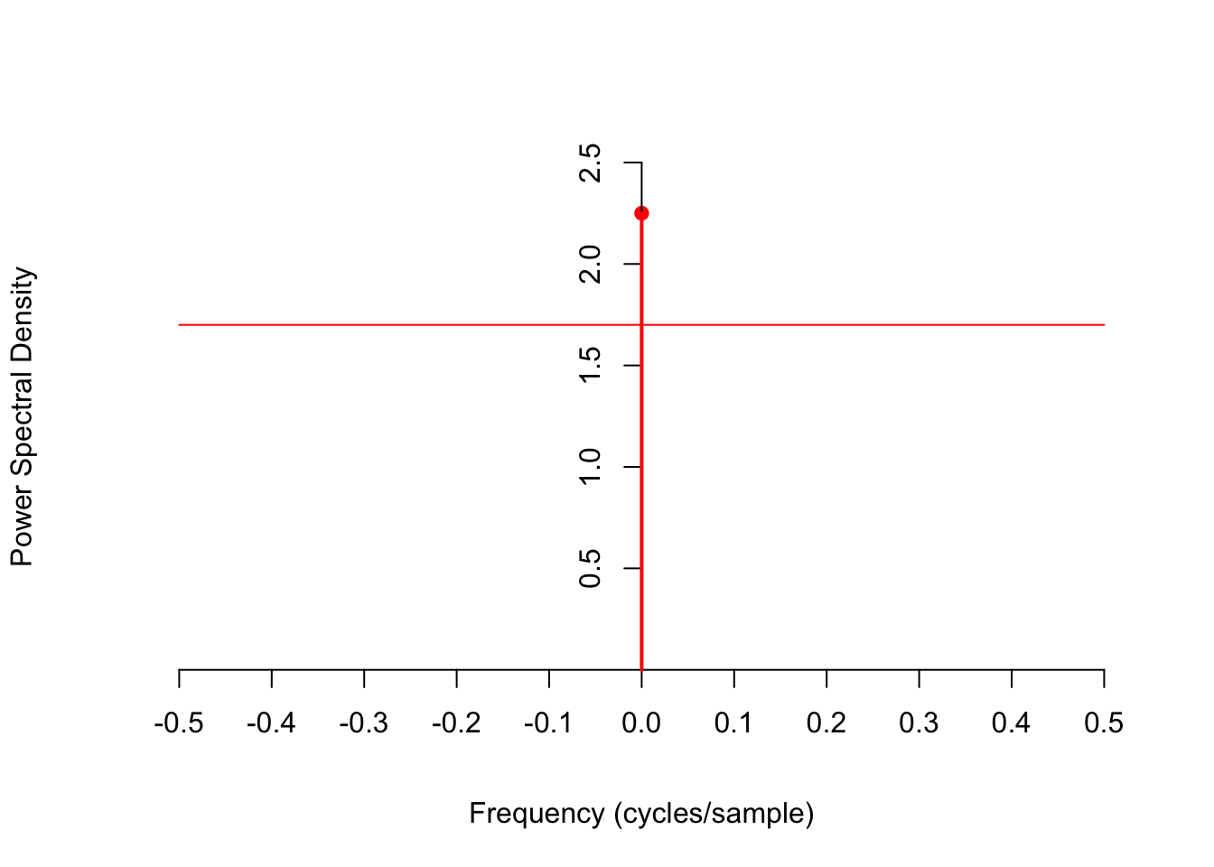
To check that we calculated the PSD correctly, we can integrate it over “all” frequencies and make sure that it matches the expected power that we obtain by evaluating the autocorrelation function at 0 (see Lesson 55). Because this is a discrete-time signal, we only integrate over frequencies below the Nyquist limit, \(|f| < 0.5\). \[ \int_{-0.5}^{0.5} S_Z(f)\,df = \int_{-0.5}^{0.5} \sigma^2\,df + \mu^2 \int_{-0.5}^{0.5} \delta(f)\,df = \sigma^2 + \mu^2 \] This matches \(R_Z[0] = \sigma^2 \delta[0] + \mu^2 = \sigma^2 + \mu^2\).
The power in this signal below 0.2 cycles/sample can be calculated by integrating the PSD over that frequency range, remembering to include both positive and negative frequencies.
\[ \int_{-0.2}^{0.2} S_Z(f)\,df = \int_{-0.2}^{0.2} \sigma^2\,df + \mu^2 \int_{-0.2}^{0.2} \delta(f)\,df = 0.4\sigma^2 + \mu^2. \]
Example 56.2 Consider the process \(\{X(t)\}\) from Example 53.5. This process is stationary, with autocorrelation function \[ R_X(\tau) = 5 e^{-\tau^2 / 3} + 4. \] The power spectral density is its Fourier transform. Using linearity, scaling, and the Continuous-Time Fourier Transform table in Appendix D.1, we see that \[\begin{align*} S_X(f) &= \mathscr{F}[5 e^{-3 \tau^2} + 4] \\ &= 5 \mathscr{F}[\underbrace{e^{-3 \tau^2}}_{e^{-\pi \left(\sqrt{\frac{3}{\pi}}\tau\right)^2}}] + 4 \mathscr{F}[1] & \text{(linearity)} \\ &= 5 \sqrt{\frac{\pi}{3}} e^{-\pi (\sqrt{\frac{\pi}{3}} f)^2} + 4 \delta(f) & \text{(scaling by $a = \sqrt{\frac{3}{\pi}}$)} \end{align*}\] Notice how we massaged \(e^{-3\tau^2}\) into the form \(e^{-\pi (a\tau)^2}\), which is a scale transform of one of the functions in Appendix D.1.
This power spectral density is graphed below. We see that this process has more power at the lower frequencies than at the higher frequencies.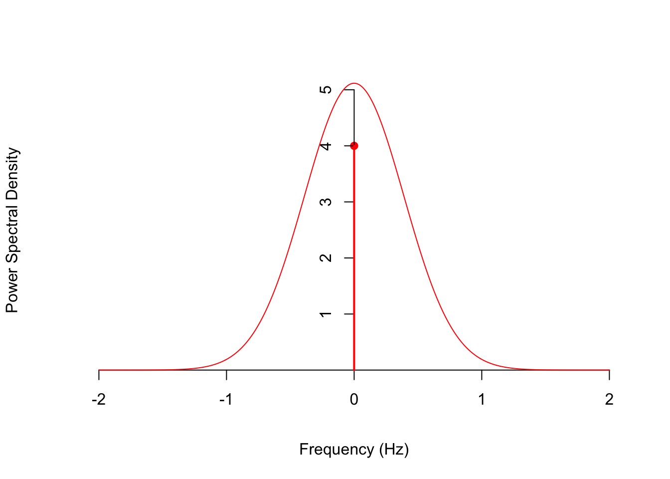
One way to check that we calculated the PSD correctly is to integrate it over all frequencies and making sure it matches the expected power we calculated in Lesson 55. \[ \int_{-\infty}^{\infty} S_X(f)\,df = \int_{-\infty}^{\infty} 5 \sqrt{\frac{\pi}{3}} e^{-\pi^2 f^2 / 3}\,df + 4 \int_{-\infty}^{\infty} \delta(f)\,df = 5 + 4 = 9. \]
The power in this signal below above 1 Hz can be calculated by integrating the PSD, remembering to include both positive and negative frequencies. Since the PSD is symmetric, the easiest way to do this is to double the integral over \(1 < f < \infty\).
\[ 2 \int_{1}^{\infty} S_X(f)\,df = 2 \int_1^{\infty} 5 \sqrt{\frac{\pi}{3}} e^{-\pi^2 f^2 / 3}\,df = .0515. \]
Essential Practice
For these questions, you may want to refer to the autocorrelation function you calculated in Lesson 54.
Radioactive particles hit a Geiger counter according to a Poisson process at a rate of \(\lambda=0.8\) particles per second. Let \(\{ N(t); t \geq 0 \}\) represent this Poisson process.
Define the new process \(\{ D(t); t \geq 3 \}\) by \[ D(t) = N(t) - N(t - 3). \] This process represents the number of particles that hit the Geiger counter in the last 3 seconds. Calculate the PSD of \(\{ D(t); t \geq 3 \}\). What is the expected power above 1 Hz?
Consider the moving average process \(\{ X[n] \}\) of Example 48.2, defined by \[ X[n] = 0.5 Z[n] + 0.5 Z[n-1], \] where \(\{ Z[n] \}\) is a sequence of i.i.d. standard normal random variables. Calculate the PSD of \(\{ X[n] \}\). What is the expected power below 0.1 cycles per sample?
Let \(\Theta\) be a \(\text{Uniform}(a=-\pi, b=\pi)\) random variable, and let \(f\) be a constant. Define the random phase process \(\{ X(t) \}\) by \[ X(t) = \cos(2\pi f t + \Theta). \] Calculate the PSD of \(\{ X(t) \}\).
Let \(\{ X(t) \}\) be a continuous-time random process with mean function \(\mu_X(t) = -1\) and autocovariance function \(C_X(s, t) = 2e^{-|s - t|/3}\). Calculate the PSD of \(\{ X(t) \}\). What is the expected power below 3 Hz?