Lesson 43 Expectations of Joint Continuous Distributions
Theory
This lesson collects a number of results about expected values of two (or more) continuous random variables. All of these results are directly analogous to the results for discrete random variables, except with sums replaced by integrals and the joint p.m.f. replaced by the joint p.d.f.
Example 43.1 Two points are chosen uniformly and independently along a stick of length 1. What is the expected distance between those two points?
Let \(X\) and \(Y\) be the two points that are chosen. The joint p.d.f. of \(X\) and \(Y\) is \[ f(x, y) = \begin{cases} 1 & 0 < x, y < 1 \\ 0 & \text{otherwise} \end{cases}. \]
We are interested in \(E[|X - Y|]\). By 2D LOTUS, this is \[\begin{align*} E[|X-Y|] &= \int_0^1 \int_0^1 |x-y| \cdot 1 \,dx\,dy \\ &= \iint_{x \geq y} (x - y)\,dx\,dy + \iint_{y > x} (y - x)\,dx\,dy \\ &= \int_0^1 \int_y^1 (x - y)\,dx\,dy + \int_0^1 \int_0^y (y - x)\,dx\,dy \\ &= \frac{1}{3}. \end{align*}\]Example 43.2 (Expected Power) Suppose a resistor is chosen uniformly at random from a box containing 1 ohm, 2 ohm, and 5 ohm resistor, and connected to live wire carrying a current (in Amperes) is an \(\text{Exponential}(\lambda=0.5)\) random variable, independent of the resistor. If \(R\) is the resistance of the chosen resistor and \(I\) is the current flowing through the circuit, then the power dissipated by the resitor is \(P = I^2 R\). What is the expected power?
The expectation \(E[P] = E[I^2 R]\) involves two random variables, so in principle, we have to use 2D LOTUS. However, because \(I\) and \(R\) are independent, we can use Theorem 43.2 to simplify the expected value and avoid double sums and integrals. \[\begin{align*} E[P] &= E[I^2 R] = E[I^2] E[R]. \end{align*}\] At this point, we cannot break up the expected value any further. However, \(E[I^2]\) and \(E[R]\) only involve one random variable.
- To calculate \(E[I^2]\), we can use LOTUS (38.1), or we can rearrange the shortcut formula for variance (39.2) to obtain \[ E[I^2] = \text{Var}[I] + E[I]^2 = \frac{1}{0.5^2} + \left(\frac{1}{0.5} \right)^2 = \frac{2}{0.5^2} = 8. \] (Note that we used the formulas for the expectation and variance of the exponential distribution.)
- To calculate \(E[R]\), we use the fact that the three resistors are equally likely to be chosen, so this is a discrete random variable: \[ E[R] = 1 \cdot \frac{1}{3} + 2 \cdot \frac{1}{3} + 5 \cdot \frac{1}{3} = \frac{8}{3} \]
Example 43.3 (Expected Arrival Times) In San Luis Obispo, radioactive particles reach a Geiger counter according to a Poisson process at a rate of \(\lambda = 0.8\) particles per second. What is the expected time that the \(r\)th particle hits the detector?
Recall from Theorem 35.2 that the interarrival times (i.e., times between arrivals) are independent \(\text{Exponential}(\lambda=0.8)\) random variables, \(T_i\). Then, the time of the \(r\)th arrival is the sum of the first \(r\) interarrival times: \[ S_r = T_1 + T_2 + \ldots + T_r. \] By linearity of expectation (and the formula for the expectation of the exponential distribution), the expected time of the \(r\)th arrival is \[\begin{align*} E[S_r] &= E[T_1] + E[T_2] + \ldots + E[T_r] \\ &= \frac{1}{0.8} + \frac{1}{0.8} + \ldots + \frac{1}{0.8} \\ &= \frac{r}{0.8}. \end{align*}\] The expected value increases with \(r\), which makes intuitive sense. We should expect to wait longer for the 10th arrival than the 2nd arrival.Essential Practice
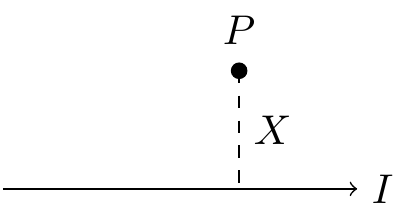
The magnetizing force \(H\) at a point \(P\), which is \(X\) meters from a wire carrying a current \(I\) (in Amperes), is given by \(H = 2I / X\). (See the figure above. This follows from the Biot-Savart Law.) Suppose that the point \(P\) is chosen randomly so that \(X\) is a continuous random variable uniformly distributed over \((3, 5)\). Assume that the current \(I\) is also a continuous random variable, uniformly distributed over \((10, 20)\). Suppose, in addition, that the random variables \(X\) and \(I\) are independent. Find the expected magnetizing force \(E[H]\).
(Hint: Use independence so that you do not have do any double integrals.)
Let \(A\) be a \(\text{Exponential}(\lambda=1.5)\) random variable, and let \(\Theta\) be a \(\text{Uniform}(a=-\pi, b=\pi)\) random variable. Assume \(A\) and \(\Theta\) are independent. Let \(s, t\) be constants, so your answers may depend on \(s, t\). Calculate:
- \(E[A \cos(\Theta + 2\pi t)]\)
- \(E[A^2 \cos^2(\Theta + 2\pi t)]\)
- \(E[A^2 \cos(\Theta + 2\pi s)\cos(\Theta + 2\pi t)]\)
(Feel free to set up the integrals and use Wolfram Alpha.)
(These calculations will come in handy later in the course.)
In a standby system, a component is used until it wears out and is then immediately replaced by another, not necessarily identical, component. (The second component is said to be “in standby mode,” i.e., waiting to be used.) The overall lifetime of a standby system is just the sum of the lifetimes of its individual components. Let \(X\) and \(Y\) denote the lifetimes of the two components of a standby system, and suppose \(X\) and \(Y\) are independent exponentially distributed random variables with expected lifetimes 3 weeks and 4 weeks, respectively. Let \(T = X + Y\), the lifetime of the standby system. What is the expected lifetime of the system?