Lesson 32 Law of Large Numbers
Motivating Example
So far, we have seen that that casino games like roulette have negative expected value (for the player). But we have also seen that there is a lot of variance. How can casinos be sure that they will not lose all of their money to players in a stroke of bad luck?
The answer lies in the Law of Large Numbers. In the long-run, as a player makes more and more negative expected value bets, it is a virtual certainty that the player will lose money.
Theory
Suppose we make the same bet repeatedly. Let \(X_i\) be our net winnings from bet \(i\). Then \(X_1, X_2, X_3, \ldots\) are independent, and furthermore, they are identically distributed (since the bets are the same). We say that \(X_1, X_2, X_3, \ldots\) are i.i.d. (which is short for “independent and identically distributed”).
Proof. Here is a heuristic proof. We calculate the expected value and the variance of \[ \bar X_n \overset{\text{def}}{=} \frac{X_1 + X_2 + \ldots + X_n}{n}. \]
The expected value is: \[\begin{align*} E[\bar X_n] &= E\left[ \frac{X_1 + X_2 + \ldots + X_n}{n} \right] \\ &= \frac{1}{n} E[X_1 + X_2 + \ldots + X_n] \\ &= \frac{1}{n} (E[X_1] + E[X_2] + \ldots + E[X_n]) \\ &= \frac{1}{n} nE[X_1] \\ &= E[X_1]. \end{align*}\]
The variance is: \[\begin{align*} \text{Var}[\bar X_n] &= \text{Var}\left[ \frac{X_1 + X_2 + \ldots + X_n}{n} \right] \\ &= \frac{1}{n^2} \text{Var}\left[ X_1 + X_2 + \ldots + X_n \right] \\ &= \frac{1}{n^2} (\text{Var}[X_1] + \text{Var}[X_2] + \ldots + \text{Var}[X_n]) \\ &= \frac{1}{n^2} n \text{Var}[X_1] \\ &= \frac{\text{Var}[X_1]}{n}. \end{align*}\]
So we see that as \(n\to\infty\), the expected value is fixed at \(E[X_1]\), and the variance approaches \(0\). A random variable with zero variance is a constant. Therefore, in the limit, the random variable \(\bar X_n\) approaches the constant \(E[X_1]\).To appreciate the Law of Large Numbers, consider betting on reds in roulette, a bet with an expected value of -$0.05, represented by a red dashed line in the figure below. There are many possible ways it could turn out; three sample paths are shown below.
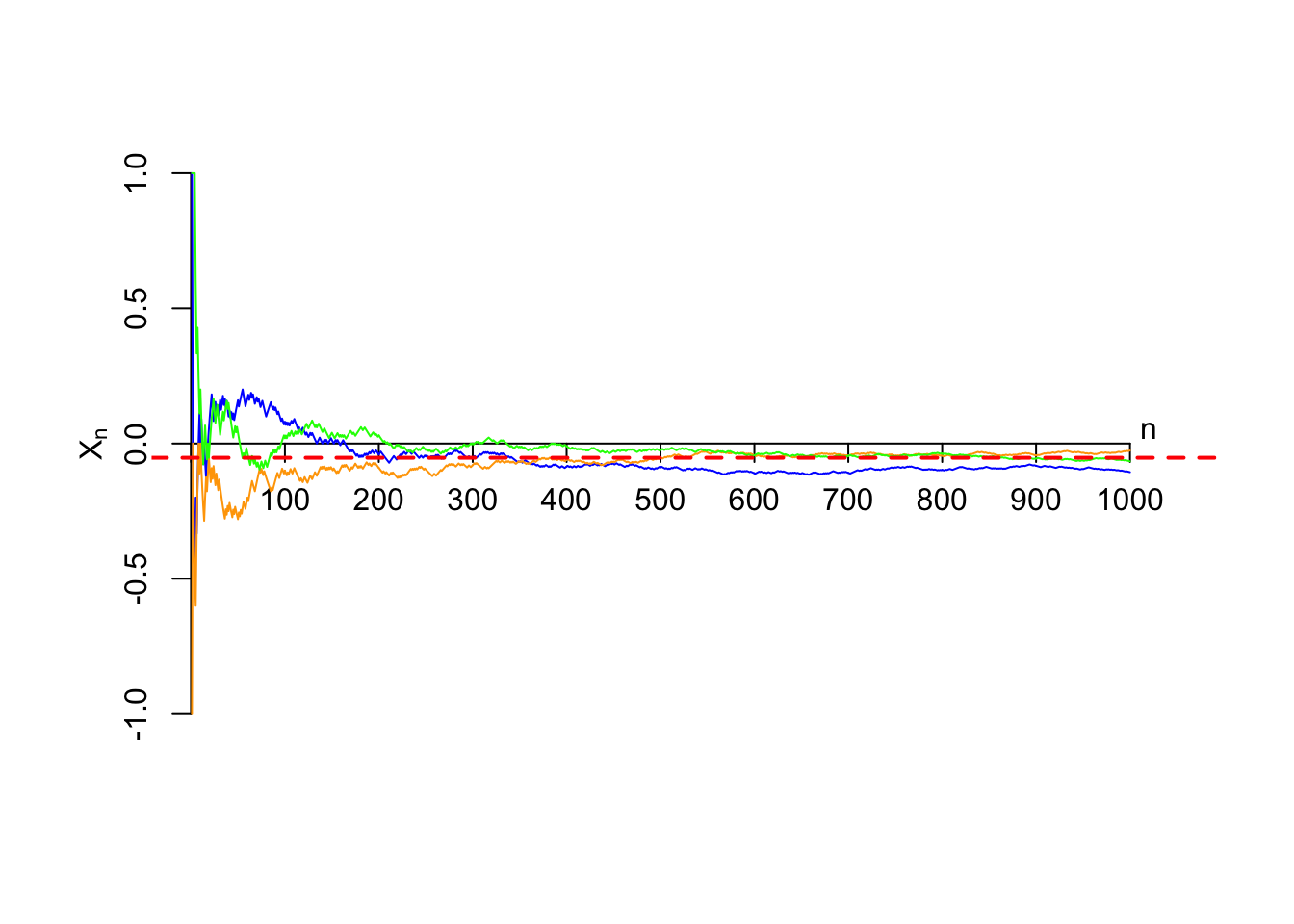
There is a lot of uncertainty about how much you will make (on average) in the first 200 bets, but by the time we have made 1000 bets, there is not much uncertainty at all. We are guaranteed to lose money in the long run. The game of chance involves very little chance, especially when you are a large casino, which handles millions of such bets every year.
Essential Practice
These questions make reference to the opening scene from the Tom Stoppard play Rosencrantz and Guildenstern are Dead (a retelling of Shakespeare’s Hamlet). You do not need to watch the scene to answer these questions, but I’ve included it just for fun.
Rosencrantz and Guildenstern have just learned the Law of Large Numbers. It turns out that they have a different understanding of what the law says…
Guildenstern: The Law of Large Numbers says that in the long run, the coin will land heads as often as it lands tails.
Rosencrantz: I don’t think that’s what it says. The Law of Large Numbers says that the fraction of heads will get closer and closer to 1/2, which is the expected value of each toss.
Guildenstern: Isn’t that the same as what I said?
Rosencrantz: No, you said, “The coin will land heads as often as it lands tails,” which implies that the difference between the number of heads and the number of tails will get smaller as we toss the coin more and more. I don’t think the number of heads will be close to the number of tails.
Guildenstern: If the fraction of heads is close to 1/2, then the number of heads must be close to the number of tails. How could it be otherwise?
Who is right: Rosencrantz or Guildenstern? Calculate the variance of \[ \text{number of heads in $n$ tosses} - \text{number of tails in $n$ tosses} \] as a function of \(n\). In light of this calculation, do you agree with Guildenstern that the difference between the number of heads and the number of tails approaches 0 as the number of tosses increases?
Rosencrantz and Guildenstern are tossing a coin. The coin has landed heads 85 times in a row. They discuss the probability that the next toss is heads.
Rosencrantz: We are due for tails! We have had so many heads that the next toss has to be more likely to land tails.
Guildenstern: Not so fast. Didn’t we call this the “gambler’s fallacy” in Lesson 7? The coin tosses are independent, so each toss is still equally likely to land heads or tails, regardless of past experience.
Rosencrantz: But what about the Law of Large Numbers? It says that we have to end up with 50% tails eventually. We are in a deep hole from the 85 heads in a row. How can we get back to 50% tails if the coin is not more likely now to land tails?
Of course, Guildenstern is right. The coin is not more likely to land tails. But how would you answer Rosencrantz’s question? Why does the Law of Large Numbers not contradict the gambler’s fallacy?