Lesson 35 Exponential Distribution

Motivating Example

In Fishtown, buses do not operate on a fixed schedule. Instead, they arrive according to a Poisson process at a rate of one per 10 minutes. How long would you have to wait if you show up at a bus stop at an arbitrary time?

Most people guess that they would have to wait about 5 minutes, since usually you will show up at the bus stop in between bus arrivals. Surprisingly, the answer is that you have to wait just as long as if you had arrived right when the previous bus was leaving! We will see why at the end of this lesson.

Theory

The exponential distribution is commonly used to model time: the time between arrivals, the time until a component fails, the time until a patient dies. We have already encountered several examples of exponential random variables—the time of the first arrival in a Poisson process follows an exponential distribution.

Definition 35.1 (Exponential Distribution) A random variable $X$ is said to follow a $\text{Exponential}(\lambda)$ distribution if its p.d.f. is \[\begin{equation} f(x) = \begin{cases} \lambda e^{-\lambda x} & x \geq 0 \\ 0 & \text{otherwise} \end{cases}, \tag{35.1} \end{equation}\] or equivalently, if its c.d.f. is \[\begin{equation} F(x) = \begin{cases} 1 - e^{-\lambda x} & x \geq 0 \\ 0 & \text{otherwise} \end{cases}. \tag{35.2} \end{equation}\]

The p.d.f. and c.d.f., for three different values of $\lambda$, are graphed below.

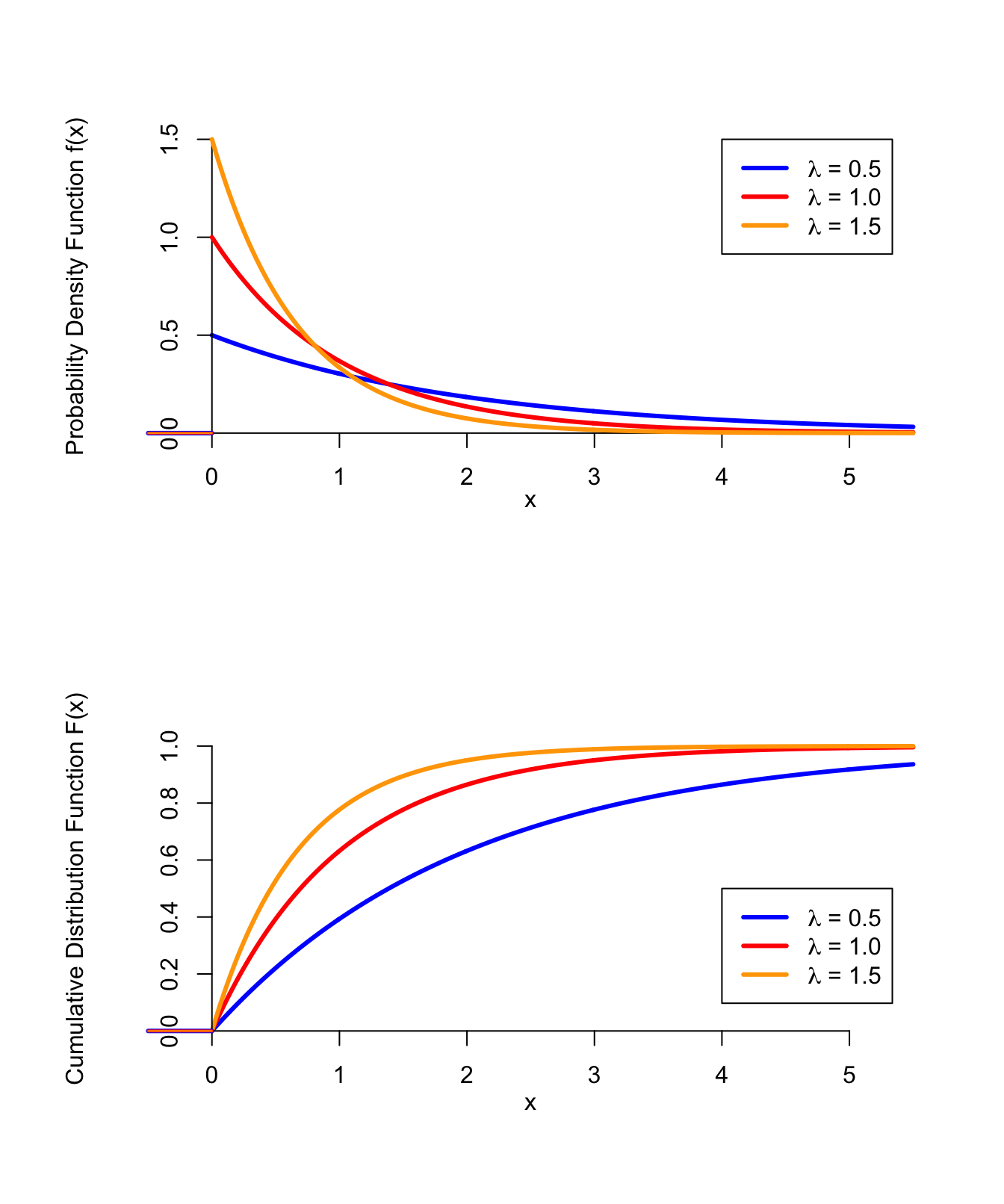
Figure 35.1: PDF and CDF of the Exponential Distribution

First, we show that the first arrival time in a Poisson process follows an exponential distribution. These calculations follow closely the ones we did in Lesson 33.

Theorem 35.1 (First Arrival Time in a Poisson Process) The time of the first arrival in a Poisson process of rate $\lambda$ is an $\text{Exponential}(\lambda)$ random variable.

Proof. Let $T$ be the time of the first arrival. Then, for $t > 0$, the c.d.f. of $T$ is \[\begin{align*} F(t) &= P(T \leq t) \\ &= 1 - P(T > t) \\ &= 1 - P(\text{0 arrivals in $(0, t)$}) \\ &= 1 - e^{- \lambda t} \frac{(\lambda t)^0}{0!} \\ &= 1 - e^{-\lambda t}. \end{align*}\] This is the c.d.f. of an $\text{Exponential}(\lambda)$ random variable, as shown in (35.2).

In fact, the time between any two arrivals in a Poisson process follows the same distribution.

Theorem 35.2 (Interarrival Times in a Poisson Process) The times between arrivals (called interarrival times) in a Poisson process of rate $\lambda$ are independent $\text{Exponential}(\lambda)$ random variables.

Proof. Let $T_1$ be the time of the first arrival and $T_2$ be the time between the first and second arrivals.

The distribution of $T_2$ given $T_1$ is \[\begin{align*} P(T_2 \leq x | T_1 = t) &= P(\text{at least 2 arrivals on $(0, t + x)$} | T_1 = t) \\ &= P(\text{at least 1 arrival on $(t, t + x)$} | T_1 = t) \\ &= P(\text{at least 1 arrival on $(t, t + x)$}) \\ &= 1 - e^{-\lambda x} \frac{(\lambda x)^0}{0!} \\ &= 1 - e^{-\lambda x}, \end{align*}\] which is the c.d.f. of an $\text{Exponential}(\lambda)$ random variable. Moreover, this expression does not depend on $t$, so $T_1$ and $T_2$ are independent, so this is also the (unconditional) distribution of $T_2$.

The key to the above proof was the third equality. $\{ T_1 = t \}$ is an event that depends on what happens on the interval $(0, t)$. But by the definition of the Poisson process, it is independent of what happens on the interval $(t, t + x)$.

By similar reasoning, we can show that $T_3$, the time between the second and third arrivals, is independent of $T_1$ and $T_2$, and so on.

The exponential distribution can be used to model random variables that have nothing to do with a Poisson process, as the next example illustrates.

Example 35.1 (Lifetime of a Lightbulb) The lifetime of a lightbulb (in years) is an $\text{Exponential}(\lambda=0.3)$ random variable. What is the probability that the lightbulb lasts between 1 and 5 years?

Solution. Let $X$ be the lifetime of the lightbulb. Then, the p.d.f. of $X$ is \[ f(x) = \begin{cases} 0.3 e^{-0.3 x} & x \geq 0 \\ 0 & x < 0 \end{cases}. \] We integrate this p.d.f. from 1 to 5: \[ P(1 < X < 5) = \int_1^5 f(x)\,dx = \int_1^5 0.3 e^{-0.3 x}\,dx \approx .517. \] Alternatively, we could have used the c.d.f. of $X$: \[ P(1 < X < 5) = F(5) - F(1) = (1 - e^{-0.3 \cdot 5}) - (1 - e^{-0.3 \cdot 1}) \approx .517. \]

Although it is not too hard to compute probabilities from the exponential distribution, we can also use software to calculate these probabilities for us. Open up this notebook in Colab and play around with it.

The exponential distribution has a surprising property called the memoryless property.

Theorem 35.3 (Memoryless Property of the Exponential Distribution) An exponential random variable $X$ has the memoryless property. That is, for any $s, t > 0$, \[\begin{equation} P(X > s + t | X > s) = P(X > t) \tag{35.3} \end{equation}\]

Proof. We use the fact that $P(X > x) = 1 - F(x) = 1 - (1 - e^{-\lambda x}) = e^{-\lambda x}$. \[\begin{align*} P(X > s + t | X > s) &= \frac{P(X > s + t \text{ and } X > s)}{P(X > s)} \\ &= \frac{P(X > s + t)}{P(X > s)} \\ &= \frac{e^{-\lambda (s + t)}}{e^{-\lambda s}} \\ &= e^{-\lambda t} \\ &= P(X > t) \end{align*}\]

The memoryless property has some surprising consequences. The example presented at the beginning of the lesson is one of them.

Example 35.2 (The Waiting Time Paradox) If buses in Fishtown arrive at a bus stop according to a Poisson process at a rate of one per 10 minutes (i.e., $\lambda = 0.1$ arrivals per minute), how long do you have to wait before the next bus arrives?

We know from Theorem 35.2 that the time $X$, between when the previous bus arrived and when the next bus will arrive, follows a $\text{Exponential}(\lambda=0.1)$ distribution. However, you showed up at the bus stop some time $s$ after the previous bus had left, so you should not have to wait as long as $X$.

Instead, your waiting time is $W = X - s$, given that $X > s$ (i.e., the next bus has not arrived yet when you show up at the stop). But by the memoryless property (35.3), \[ P(W > t | X > s) = P(X - s > t | X > s) = P(X > t). \] So you have to wait just as long as if you had showed up right as the previous bus was leaving. You do not save any time by showing up in between bus arrivals!

Essential Practice

Let $X$ denote the distance (in meters) that an animal moves from its birth site to the first territorial vacancy it encounters. Suppose that for banner-tailed kangaroo rats, $X$ has an exponential distribution with parameter $\lambda = .01386$ (as suggested in the article “Competition and Dispersal from Multiple Nests,” Ecology, 1997: 873–883).
1. What is the probability that the distance is more than 100 m?
2. This probability is higher than it was in 1950, due to environmental changes. Suppose that in 1950, only 12% of banner-tailed kangaroo rats moved more than 100 m from their birth site. What was the value of $\lambda$ then?
Small aircraft arrive at San Luis Obispo airport according to a Poisson process at a rate of 6 per hour.
1. What is the probability that more than 15 minutes elapse before the first plane lands?
2. What is the probability that more than 15 minutes elapse between when the first and second planes land?
3. What is the probability that it takes more than 15 minutes elapse before the first plane lands and more than 15 minutes elapse between when the first and second planes land?
4. What is the probability that more than 30 minutes elapse before two planes have landed? Why is the answer different than your answer to part c? (Hint: You can calculate this using properties of a Poisson process. Rewrite the event in terms of the number of planes that land in the interval $(0, 30)$.)
A post office has 2 clerks. Alice enters the post office while 2 other customers, Bob and Claire, are being served by the 2 clerks. She is next in line. Assume that the time a clerk spends serving a customer (in minutes) follows an $\text{Exponential}(\lambda=0.2)$ distribution. What is the probability that Alice is the last of the 3 customers to be done being served? (Hint: This can be answered without any calculations, by thinking about the memoryless property.)