Lesson 11 Cumulative Distribution Functions
Theory
The p.m.f. 10.1 is one way to describe a random variable, but it is not the only way. The cumulative distribution function is a different representation that contains the same information as the p.m.f.
Example 11.1 (Calculating the C.D.F.) Let’s calculate the c.d.f. of \(X\), the number of diamonds among the community cards, using the p.m.f. that we calculated in Lesson 10. Note that \(F(x)\) is the sum of all the probabilities up to \(x\). So, for example, \[\begin{align*} F(2.8) = P(X \leq 2.8) &= f(0) + f(1) + f(2) \\ &= .2546 + .4243 + .2496 \\ &= .9284. \end{align*}\] There is no simple formula for \(F(x)\). However, we can describe it piecewise. \[ F(x) = \begin{cases} 0 & x \leq 0 \\ .2546 & 0 \leq x < 1 \\ .6788 & 1 \leq x < 2 \\ .9284 & 2 \leq x < 3 \\ .9926 & 3 \leq x < 4 \\ .9997 & 4 \leq x < 5 \\ 1.0 & x \geq 5 \end{cases}. \] Note that the c.d.f. of \(X\) has the following properties:
- It is constant between integers. Because it is impossible for the random variable \(X\) to assume non-integer values, \(F(1.2) = P(X \leq 1.2)\) and \(F(1) = P(X \leq 1)\) must be the same.
- The value of \(F(x)\) increases from 0 to 1 as \(x\) increases. This makes sense because as \(x\) increases, we accumulate more and more probability.
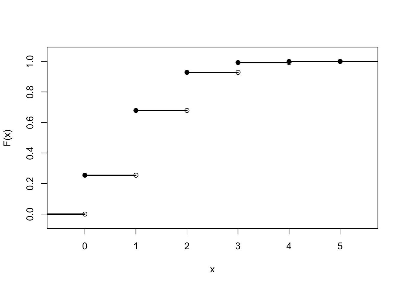
Figure 11.1: Graph of a cumulative distribution function
Note that the c.d.f. \(F(x)\) can be evaluated at all values \(x\), not just at integer values.
Example 11.3 (Using the C.D.F.) Some probabilities are easier to calculate using the c.d.f. than using the p.m.f. For example, the probability that Alice gets a flush, \(P(X \geq 3)\), can be calculated by using the complement rule (5.2) and looking up the appropriate probability directly from the c.d.f. \(F(x)\).
\[\begin{align*} P(X \geq 3) &= 1 - P(X < 3) \\ &= 1 - P(X \leq 2) \\ &= 1 - F(2) \\ &= 1 - .9284 \\ &= .0716 \end{align*}\]
Remember that the c.d.f. \(F(x)\) always includes the probability of \(x\). Since \(P(X < 3)\) should not include the probability of \(3\), we use \(F(2)\) instead of \(F(3)\).
At the beginning of this lesson, we mentioned that the c.d.f. contains the exact same information as the p.m.f., no more and no less. Therefore, it should be possible to recover the p.m.f. from the c.d.f.
For example, how would we calculate \(f(3) = P(X = 3)\), if we only knew the c.d.f. \(F(x)\)? We could subtract \(P(X \leq 2)\) from \(P(X \leq 3)\) to get just the probability that it is equal to 3. \[\begin{align*} f(3) = P(X = 3) &= P(X \leq 3) - P(X \leq 2) \\ &= F(3) - F(2) \\ &= .9926 - .9284 \\ &= .0642, \end{align*}\] which agrees with the p.m.f. from Lesson 10.Examples
Continuing with the example from the lesson, let \(Y\) be the number of Jacks among the community cards. Calculate and graph the c.d.f. of \(Y\).
Consider a random variable \(Z\) with c.d.f. given by the formula \[\begin{align*} F(x) &= \begin{cases} 1 - 3^{-\lfloor x \rfloor} & x \geq 0 \\ 0 & \text{otherwise} \end{cases}. \end{align*}\] (Note that \(\lfloor x \rfloor\) denotes the floor operator, which rounds \(x\) down to the nearest integer. So \(\lfloor 3.9 \rfloor = 3\) and \(\lfloor 7.1 \rfloor = 7\).)
Graph the c.d.f. \(F(x)\). Then, use it to calculate:- \(P(Z > 3)\)
- \(P(Z = 2)\)