Lesson 17 Poisson Process
Motivating Example
A Geiger counter is a device used for measuring radiation in the atmosphere. Each time it detects a radioactive particle, it makes a clicking sound. In the figure below, the orange points below indicate the times at which the Geiger counter detected a radioactive particle.
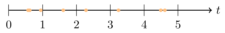
Figure 17.1: Radioactive Particles Reaching a Geiger Counter
The radioactive particles hit the Geiger Counter at seemingly random and unpredictable times. In this lesson, we learn to make sense of the randomness.
Theory
Radioactive particles are a classic example of a type of random process called the Poisson process. The Poisson process is used to model random events, called “arrivals”, over time.
Definition 17.1 (Poisson Process) A Poisson process of rate \(\lambda\) is characterized by the following properties:
- The number of arrivals in any interval \((t_0, t_1)\) follows a Poisson distribution with \(\mu = \lambda (t_1 - t_0)\). That is, the parameter \(\mu\) increases proportionally to the length of the interval.
- The numbers of arrivals in non-overlapping intervals are independent.
These two properties allow us to calculate any probability of interest.
Example 17.1 (Geiger Counter) In San Luis Obispo, radioactive particles reach a Geiger counter according to a Poisson process at a rate of \(\lambda = 0.8\) particles per second.
- What is the probability that the Geiger counter detects 3 or more particles in the next 4 seconds?
- What is the probability that the Geiger counter detects (exactly) 1 particle in the next second and 3 or more in the next 4 seconds?
Solution. .
- The number of particles arriving at the detector in the next 4 seconds, \(X\), follows a \(\text{Poisson}(\mu = 0.8 \cdot (4 - 0) = 3.2)\) distribution by Property 1 (17.1). Therefore, the probability of detecting 3 or more particles is: \[\begin{align*} P(X \geq 3) &= 1 - P(X < 3) \\ &= 1 - f(0) - f(1) - f(2) \\ &= 1 - e^{-3.2} \frac{3.2^0}{0!} - e^{-3.2} \frac{3.2^1}{1!} - e^{-3.2} \frac{3.2^2}{2!} \\ &\approx .6201 \end{align*}\]
The joint probability \[ P(\text{1 particle in (0, 1)} \text{ AND } \text{3 or more particles in (0, 4)}) \] involves two events that are not independent. However, we can rewrite the joint probability as: \[ P(\text{1 particle in (0, 1)} \text{ AND } \text{2 or more particles in (1, 4)}). \] Now, \((0, 1)\) and \((1, 4)\) are non-overlapping intervals, so the number of particles arriving in \((0, 1)\) is independent of the number of particles arriving in \((1, 4)\) by Property 2 (17.1). Therefore, by Theorem 7.1, we obtain their joint probability by multiplying their individual probabilities: \[ P(\text{1 particle in (0, 1)}) \cdot P(\text{2 or more particles in (1, 4)}). \]
Now, we know from Property 1 (17.1) that
- the number of particles in \((0, 1)\) follows a \(\text{Poisson}(\mu = 0.8)\) distribution, and
- the number of particles in \((1, 4)\) follows a \(\text{Poisson}(\mu = 2.4)\) distribution.
We can also calculate these probabilities with the aid of software:
## 0.24858997647262118Why Poisson?
Why does it make sense to assume that the number of arrivals on any interval follows a Poisson distribution? If we chop time up into tiny segments of length \(\Delta t\), then the probability of an arrival on any one of these segments will be small—but there will be many such intervals.
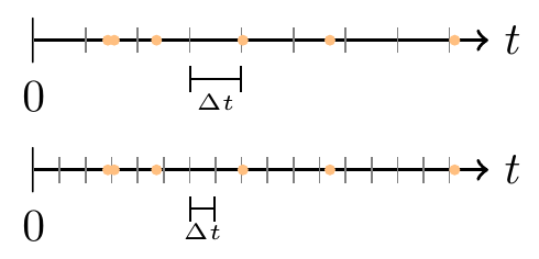
Figure 17.2: Chopping Up Time in a Poisson Process
If we further assume that arrivals are independent across these tiny segments, then the number of arrivals follows a binomial distribution, with large \(n\) (because there are many segments) and small \(p\) (because an arrival is unlikely to fall exactly in any given segment). We saw in Theorem 16.1 that the Poisson distribution is a good approximation to the binomial when \(n\) is large and \(p\) is small.
Technical Detail: In order for the number of arrivals to be binomial, each tiny segment must contain either 1 arrival or none; there cannot be 2 or more arrivals in any segment. Usually, if \(\Delta t\) is so small that it is rare to get even 1 arrival in a segment, then it is essentially impossible to get 2 arrivals.
Essential Practice
Packets arrive at a certain node on the university’s intranet at 10 packets per minute, on average. Assume packet arrivals meet the assumptions of a Poisson process.
- Calculate the probability that exactly 15 packets arrive in the next 2 minutes.
- Calculate the probability that more than 60 packets arrive in the next 5 minutes.
- Calculate the probability that the next packet will arrive in within 15 seconds.
Small aircraft arrive at San Luis Obispo airport according to a Poisson process at a rate of 6 per hour.
- What is the probability that exactly 5 small aircraft arrive in the first hour (after opening) and exactly 7 arrive in the hour after that?
- What is the probability that fewer than 5 small aircraft arrive in the first hour and at least 10 arrive in the hour after that?
- What is the probability that exactly 5 small aircraft arrive in the first hour and exactly 12 aircraft arrive in the first two hours?