Lesson 42 Marginal Continuous Distributions
Motivating Example
In Lesson 40 on the normal distribution, we saw that there is no closed-form expression for the antiderivative \[ \int ce^{-z^2/2}\,dz, \] where \(c\) is a constant. The definite integral must be computed numerically. This means that we can compute the integral to any precision we like, but exact values are, in general, impossible.
How, then, can we be sure that the constant \(c\) must be \(1 / \sqrt{2\pi}\) for the total probability to be 1? That is, \[\begin{equation} \int_{-\infty}^\infty \frac{1}{\sqrt{2\pi}} e^{-z^2/2}\,dz = 1. \tag{42.1} \end{equation}\] Using numerical integration, we might be able to figure out that \(c \approx .3989423\) (or as many decimal places as desired), but how do we know it is \(1 / \sqrt{2\pi}\) exactly?
It turns out that the definite integral (42.1) can be evaluated exactly, but to see this, we need to use joint distributions.
Theory
The definition for the marginal p.d.f. mirrors the definition of the marginal p.m.f. for discrete distributions 19.1, except with sums replaced by integrals and the joint p.m.f. replaced by the joint p.d.f.If \(X\) and \(Y\) are independent, then their joint p.d.f. is the product of their marginal p.d.f.s, just like it was for discrete random variables (Theorem 19.1):
In the following examples, we construct the joint p.d.f. of two independent random variables \(X\) and \(Y\) using Theorem 42.1. Then, we integrate the joint p.d.f. to obtain probabilities, as usual.
Example 42.1 (Symmetry of Continuous Random Variables) The lifetimes of two lightbulbs, \(X\) and \(Y\), are independent \(\text{Exponential}(\lambda)\) random variables. What is the probability the second lightbulb lasts longer than the first, \(P(Y > X)\)?
First, we write down the joint p.d.f. using Theorem 42.1: \[ f(x, y) = \begin{cases} \lambda e^{-\lambda x} \cdot \lambda e^{-\lambda y} & x, y \geq 0 \\ 0 & \text{otherwise} \end{cases}. \] Now, we just need to integrate this p.d.f. over the region where \(y > x\). We sketch a bird’s-eye view below.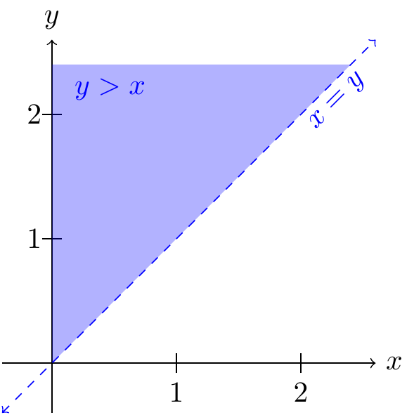
Now we integrate over the above region: \[\begin{align*} P(Y > X) &= \int_0^\infty \int_x^\infty \lambda^2 e^{-\lambda x - \lambda y}\,dy\,dx \\ &= \int_0^\infty \lambda e^{-\lambda x} \underbrace{\int_x^\infty \lambda e^{-\lambda y}\,dy}_{e^{-\lambda x}}\,dx \\ &= \int_0^\infty \lambda e^{-\lambda x} e^{-\lambda x}\,dx \\ &= \int_0^\infty \lambda e^{-2\lambda x}\,dx \\ &= \frac{1}{2}. \end{align*}\] (One way to see the last equality is to recognize \(f(x) = 2 \lambda e^{-2\lambda x}; x > 0\) as the p.d.f. of an \(\text{Exponential}(2\lambda)\) distribution, so we multiply and divide by \(2\) to make the integrand match this p.d.f., which then must integrate to 1.)
In hindsight, the probability has to be \(1/2\) by symmetry. We know that either \(X > Y\) or \(X < Y\), since the probability that \(X = Y\) (i.e., the two lightbulbs have exactly the same lifetime) is zero. Because \(X\) and \(Y\) are independent with the same distribution, there is no reason for one to be preferred over another, so \(P(X > Y) = P(X < Y) = \frac{1}{2}\). In fact, by the exact same argument, this is true for all independent and identically distributed (i.i.d.) continuous random variables with a joint p.d.f. ```
The last example answers the question posed at the beginning of this lesson.
Example 42.2 (The Gaussian Integral) The p.d.f. of a standard normal random variable \(Z\) is \[ f(z) = c e^{-z^2/2}, \] where \(c\) is a constant to make the p.d.f. integrate to 1.
Surprisingly, the easiest way to determine \(c\) is to define two independent standard normal random variables \(X\) and \(Y\), and use the fact that their joint p.d.f. must integrate to 1. By Theorem 42.1, the joint p.d.f. of \(X\) and \(Y\) is \[ f(x, y) = ce^{-x^2 /2} \cdot ce^{-y^2 / 2} = c^2 e^{-(x^2 + y^2) / 2}. \] We know from Lesson 41 that the total volume under any joint p.d.f. must be 1: \[ 1 = \int_{-\infty}^\infty \int_{-\infty}^\infty f(x, y)\,dx\,dy = \int_{-\infty}^\infty \int_{-\infty}^\infty c^2 e^{-(x^2 + y^2) / 2}\,dx\,dy. \] Surprisingly, this double integral can be evaluated (even though the single integral could not). To evaluate the double integral, we convert to polar coordinates, using the substitutions \(r^2 = x^2 + y^2\) and \(dx\,dy = r\,dr\,d\theta\): \[\begin{align*} c^2 \int_{-\infty}^\infty \int_{-\infty}^\infty e^{-(x^2 + y^2) / 2}\,dx\,dy &= c^2 \int_{0}^{2\pi} \int_{0}^\infty e^{-r^2 / 2} r\,dr\,d\theta \\ &= c^2 \int_0^{2\pi} \underbrace{\int_0^\infty e^{-u}\,du}_{1} \,d\theta & \text{(using $u=r^2/2$)} \\ &= c^2 (2\pi). \end{align*}\] Setting this equal to 1, we see that \(c^2 = \frac{1}{2\pi}\). In other words, \(c = \frac{1}{\sqrt{2\pi}}\).Essential Practice
Let \(X\) and \(Y\) be continuous random variables with joint p.d.f. \[ f(x, y) = \begin{cases} \frac{1}{12} (1 + \frac{1}{18}(x - 2)(2y - 3)) & 0 < x < 4, 0 < y < 3 \\ 0 & \text{otherwise} \end{cases}. \]
- Find the marginal p.d.f.s of \(X\) and \(Y\). Are these named distributions? (Feel free to set up and the integral and use Wolfram Alpha to do the rest.)
- Are \(X\) and \(Y\) independent? (Hint: According to Theorem 42.1, what would their joint p.d.f. have to be if they were independent?)
- Harry and Sally independently go to Katz’s Deli for lunch on weekdays from their
respective jobs. Let \(H\) be the time that Harry arrives and \(S\) be the time that
Sally arrives (in minutes after 12 p.m.). \(H\) and \(S\)
are independent \(\text{Uniform}(a=0, b=90)\) random variables.
- What is the joint p.d.f. of \(H\) and \(S\)? Sketch a bird’s-eye view of the joint p.d.f.
If they each take 20 minutes to eat their lunch after they arrive, what is the probability that Harry meets Sally…?
(Hint: The two are able to meet if they arrive within 20 minutes of each other. Sketch the region of times that correspond to Harry and Sally meeting. You can calculate this probability by geometry, without using integration.)What is the probability that Harry arrives after Sally arrives?