Lesson 26 Linearity of Expectation
Theory
In this lesson, we learn a shortcut for calculating expected values of the form \[ E[aX + bY]. \] In general, evaluating expected values of functions of random variables requires LOTUS. But when the function is linear, we can break up the expected value into more manageable parts.
Here is an example illustrating how Theorem 26.1 can be used.
Example 26.1 (Expected Values in Roulette) In roulette, betting on a single number pays 35-to-1. That is, for each $1 you bet, you win $35 if the ball lands in that pocket.
If we let \(X\) represent your net winnings (or losses) on this bet, its p.m.f. is \[ \begin{array}{r|cc} x & -1 & 35 \\ \hline f_X(x) & 37/38 & 1/38 \end{array}. \]
In Lesson 22, we calculated \(E[X]\) directly. Here is another way we can calculate it using Theorem 26.1. Let us define a new random variable \(W\), which takes on the values 0 and 1 with the same probabilities: \[ \begin{array}{r|cc} w & 0 & 1 \\ \hline f_W(w) & 37/38 & 1/38 \end{array}. \] We can think of \(W\) as an indicator variable for whether or not we win. It is easy to see that \(E[W] = 1/38\). (One way is to just use the formula. Another is to note that \(W\) is a \(\text{Binomial}(n=1, p=1/38)\) random variable, so \(E[W] = np = 1/38\).)
Now, the amount we win, \(X\), is related to this indicator variable, \(W\), by: \[ X = 36 W - 1. \] (Verify that \(X\) takes on the values \(35\) and \(-1\) with the correct probabilities.) Now, by Theorem 26.1, the expected value is \[ E[X] = E[36W - 1] = 36 E[W] - 1 = 36 \left( \frac{1}{38} \right) - 1 = -\frac{2}{38}, \] which matches what we got in Lesson 22.The next result is even more useful.
Proof. Since \(E[X + Y]\) involves two random variables, we have to evaluate the expectation using 2D LOTUS (25.1), with \(g(x, y) = x + y\). Suppose that the joint distribution of \(X\) and \(Y\) is \(f(x, y)\). Then: \[\begin{align*} E[X + Y] &= \sum_x \sum_y (x + y) f(x, y) & \text{(2D LOTUS)} \\ &= \sum_x \sum_y x f(x, y) + \sum_x \sum_y y f(x, y) & \text{(break $(x + y) f(x, y)$ into $x f(x, y) + y f(x, y)$)} \\ &= \sum_x x \sum_y f(x, y) + \sum_y y \sum_x f(x, y) & \text{(move term outside the inner sum)} \\ &= \sum_x x f_X(x) + \sum_y y f_Y(y) & \text{(definition of marginal distribution)} \\ &= E[X] + E[Y] & \text{(definition of expected value)}. \end{align*}\]
In other words, linearity of expectation says that you only need to know the marginal distributions of \(X\) and \(Y\) to calculate \(E[X + Y]\). Their joint distribution is irrelevant.
Let’s apply this to the Xavier and Yolanda problem from Lesson 18.
Example 26.2 (Xavier and Yolanda Revisited) Xavier and Yolanda head to the roulette table at a casino. They both place bets on red on 3 spins of the roulette wheel before Xavier has to leave. After Xavier leaves, Yolanda places bets on red on 2 more spins of the wheel. Let \(X\) be the number of bets that Xavier wins and \(Y\) be the number that Yolanda wins.
In Lesson 25, we calculated \(E[Y - X]\), the expected number of additional times that Yolanda wins, by applying 2D LOTUS to the joint p.m.f. of \(X\) and \(Y\). The calculation was tedious.
In this lesson, we see how linearity of expectation allows us to avoid tedious calculations. First, by (26.1) and (26.3), we see that: \[ E[Y - X] = E[Y] + E[-1 \cdot X] = E[Y] + (-1) E[X] = E[Y] - E[X]. \] We know that \(Y\) is \(\text{Binomial}(n=5, N_1=18, N_0=20)\) and \(X\) is \(\text{Binomial}(n=3, N_1=18, N_0=20)\). \(X\) and \(Y\) are definitely not independent, since three of Yolanda’s bets are identical to Xavier’s. But linearity of expectation says that to calculate \(E[Y - X]\), it does not matter how \(X\) and \(Y\) are related to each other; we only need their marginal distributions.
From Appendix A.1 (and Lesson 22), we know the expected value of a binomial random variable is \(n\frac{N_1}{N}\), so \[ E[Y - X] = E[Y] - E[X] = 5\frac{18}{38} - 3\frac{18}{38} = 2\frac{18}{38} \approx .947, \] which matches the answer we got in Lesson 25 by applying 2D LOTUS.Linearity allows us to calculate the expected values of complicated random variables by breaking them into simpler random variables.
Example 26.3 (Expected Value of the Binomial and Hypergeometric Distributions) In Lesson 22, we showed that the expected values of the binomial and hypergeometric distributions are the same: \(n\frac{N_1}{N}\). But the proofs we gave were tedious and did not give any insight into why this formula is true. Let’s prove this formula using linearity of expectation.
If \(X\) is a \(\text{Binomial}(n, N_1, N_0)\) random variable, then we can break \(X\) down into the sum of simpler random variables: \[ X = Y_1 + Y_2 + \ldots + Y_n, \] where \(Y_i\) represents the outcome of the \(i\)th draw from the box. So \(Y_i\) equals \(1\) with probability \(N_1/N\) and is \(0\) otherwise. Its p.m.f. is about as simple as it gets: \[\begin{equation} \begin{array}{rcc} y & 0 & 1 \\ \hline f(y) & N_0/N & N_1/N \end{array}. \label{eq:bernoulli_pmf} \end{equation}\]
By linearity of expectation: \[ E[X] = E[Y_1] + E[Y_2] + \ldots + E[Y_n]. \] We have taken a complicated random variable \(X\) and broken it down into simpler random variables \(Y_i\), whose expected value is trivial to calculate: \[ E[Y_i] = 0 \cdot \frac{N_0}{N} + 1 \cdot \frac{N_1}{N} = \frac{N_1}{N}. \] Therefore, \[ E[X] = \underbrace{\frac{N_1}{N} + \frac{N_1}{N} + \ldots + \frac{N_1}{N}}_{\text{$n$ terms}} = n \frac{N_1}{N}. \]
What if \(X\) is a \(\text{Hypergeometric}(n, N_1, N_0)\) random variable? We can break \(X\) down in exactly the same way, as sum of the outcomes of each draw: \[ X = Y_1 + Y_2 + \ldots + Y_n, \] except that now the \(Y_i\)s are not independent. However, each \(Y_i\) still represents a random draw from a box with \(N_1\) \(\fbox{1}\)s and \(N_0\) \(\fbox{0}\)s, so \(Y_i\) equals 1 with probability \(N_1/N\), just as before.Also, linearity of expectation does not care whether or not the random variables are independent. So the expected value of the hypergeometric is also: \[ E[X] = \underbrace{\frac{N_1}{N} + \frac{N_1}{N} + \ldots + \frac{N_1}{N}}_{\text{$n$ terms}} = n \frac{N_1}{N}. \]
Here is a clever application of linearity.
Example 26.4 Let \(X\) be a \(\text{Binomial}(n, N_1, N_0)\) random variable. What is \(E[X(X-1)]\)? In Example 24.3, we calculated this expected value using LOTUS. Here is a way to calculate it using linearity.
Remember that \(X\) represents the number of \(\fbox{1}\)s in our sample. The random variable \(X(X-1)\) then represents the number of (ordered) ways to choose two tickets from the \(\fbox{1}\)s in our sample. In the diagram below, \(n=4\) and \(X=3\). Each arrow represents one of the \(n(n-1) = 12\) ways to choose two tickets from the \(n\) tickets in the sample. The red arrows represent the \(X(X-1) = 6\) ways of choosing two tickets among the \(\fbox{1}\)s.
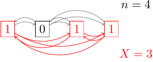
Let’s define an indicator variable \(Y_{ij}, i\neq j\) for each of the \(n(n-1)\) ways of choosing two tickets from our sample. Let \(Y_{ij}\) be 1 if tickets \(i\) and \(j\) are both \(\fbox{1}\)s. In other words, \(Y_{ij} = 1\) if and only if there is a red arrow connecting the two tickets in the diagram above.
Since \(X(X-1)\) is the number of red arrows, we have \[ X(X-1) = \sum_{i=1}^n \sum_{j\neq i} Y_{ij}. \] Now, by linearity: \[ E[X(X-1)] = \sum_{i=1}^n \sum_{j\neq i} E[Y_{ij}]. \] But \(E[Y_{ij}]\) is simply the probability that tickets \(i\) and \(j\) are both \(\fbox{1}\)s. This probability is \(E[Y_{ij}] = \frac{N_1^2}{N^2}\). Since there are \(n(n-1)\) \(Y_{ij}\)s, \[ E[X(X-1)] = n(n-1) \frac{N_1^2}{N^2}, \] which matches the answer we got in Lesson 24 by more tedious means.
Essential Practice
Each year, as part of a “Secret Santa” tradition, a group of 4 friends write their names on slips of papers and place the slips into a hat. Each member of the group draws a name at random from the hat and must by a gift for that person. Of course, it is possible that they draw their own name, in which case they buy a gift for themselves. What is the expected number of people who draw their own name?
Hint: Express this complicated random variable as a sum of indicator random variables (i.e., that only take on the values 0 or 1), and use linearity of expectation.
McDonald’s decides to give a Pokemon toy with every Happy Meal. Each time you buy a Happy Meal, you are equally likely to get any one of the 6 types of Pokemon. What is the expected number of Happy Meals that you have to buy until you “catch ’em all”?
Hint: Express this complicated random variable as a sum of geometric random variables, and use linearity of expectation.
A group of 60 people are comparing their birthdays (as usual, assume that their birthdays are independent, all 365 days are equally likely, etc.). Find the expected number of days in the year on which at least two of these people were born.
Hint: Express this complicated random variable as a sum of indicator random variables, and use linearity of expectation.
Additional Practice
A hash table is a commonly used data structure in computer science, allowing for fast information retrieval. For example, suppose we want to store some people’s phone numbers. Assume that no two of the people have the same name. For each name \(x\), a hash function \(h\) is used, where \(h(x)\) is the location to store x’s phone number. After such a table has been computed, to look up \(x\)’s phone number one just recomputes \(h(x)\) and then looks up what is stored in that location.
Typically, \(h\) is chosen to be (pseudo)random. Suppose there are 100 people, with each person’s phone number stored in a random location (independently), represented by an integer between 1 and 1000. It then might happen that one location has more than one phone number stored there, if two different people \(x\) and \(y\) end up with the same random location for their information to be stored.
Find the expected number of locations with no phone numbers stored, the expected number with exactly one phone number, and the expected number with more than one phone number.
Calculate \(E[X(X-1)]\) for a \(\text{Hypergeometric}(n, N_1, N_0)\) random variable \(X\) using linearity. (Hint: Follow Example 26.4.)