Lesson 22 Expected Value

Motivating Example

A bet on a single number in roulette has a $1/38$ chance of success. We would not play this game if we were only offered a 1-to-1 payout on this bet—that is, a chance to win $1 for each $1 we wager. What would the payout have to be to make this game fair?

Theory

So far in this class, we have described random variables by their p.m.f. or their c.d.f. These functions contain everything there is to know about the random variable. However, the p.m.f. or c.d.f. is too much information in most applications. If we want to summarize a random variable by a single number, the expected value is usually the right choice.

Definition 22.1 (Expected Value) Let $X$ be a random variable with p.m.f. $f(x)$. Then, the expected value of $X$, symbolized $E[X]$ is defined as \[\begin{equation} E[X] \overset{\text{def}}{=} \sum_x x \cdot f(x). \tag{22.1} \end{equation}\]

The expected value is a weighted average of the possible values of a random variable, where the weights are the probabilities.

How do we interpret the expected value? The next example explores this question.

Example 22.1 (Betting on a Number in Roulette) In roulette, betting on a single number pays 35-to-1. That is, for each $1 you bet, you win $35 if the ball lands in that pocket.

If we let $X$ represent your net winnings (or losses) on this bet, its p.m.f. is \[ \begin{array}{r|cc} x & -1 & 35 \\ \hline f(x) & 37/38 & 1/38 \end{array}. \]

Now, let’s calculate the expected value of this random variable. \[ E[X] = -1 \cdot \frac{37}{38} + 35 \cdot \frac{1}{38} = -0.053. \]

How do we interpret the expected value of -0.053? It is not even possible for our net winnings to be -$0.053 on this bet, since our net winnings can only be -$1 or $35. Instead, this -$0.053 represents a long-run average. If we were to repeatedly make the same bet at the roulette wheel, then we will win some and lose some. The amount that we win per bet will approach -$0.053 as we make more and more bets. This is illustrated in Figure 22.1.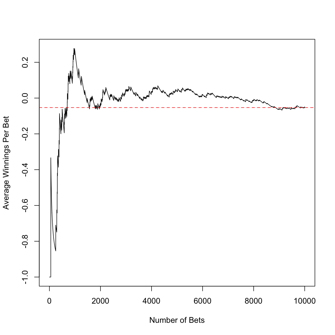

Figure 22.1: The first 50 bets were all losses, so the average winnings starts at -1. In the long run, it approaches the expected value of -.053, shown in red.

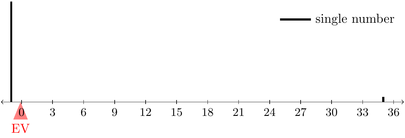
The expected value can also be interpreted as the center of mass. If we imagine the p.m.f. as resting on a scale, then the expected value is the pivot point where the scale will perfectly balance.

Figure 22.2: Expected Value as Center of Mass

Theorem 22.1 (Expected Value as Center of Mass) The expected value of a random variable $X$ with p.m.f. $f(x)$ is the center of mass of the p.m.f.

Proof. Each mass contributes torque around the pivot. Torque is mass times distance from the pivot. In order for the beam to balance at a pivot, the total torque around that pivot must be zero. We show that the total torque is zero when the pivot is chosen to be the expected value $E[X]$. \[\begin{align*} \text{torque} &= \sum \text{mass} \cdot (\text{distance from pivot}) \\ &= \sum_x f(x) \cdot (x - E[X]) \\ &= \underbrace{\sum_x f(x) \cdot x}_{E[X]} - \underbrace{\sum_x f(x)}_{1} \cdot E[X] \\ &= E[X] - E[X] \\ &= 0. \end{align*}\]

Now let’s answer the question posed at the beginning of the lesson. Although the casino’s payout of 35-to-1 is better than a 1-to-1 payout, it is still unfavorable to us. What would the payout need to be to make the game fair? In other words, we will let the p.m.f. be \[ \begin{array}{r|cc} x & -1 & c \\ \hline f(x) & 37/38 & 1/38 \end{array}, \] where $c$ is chosen to make the expected value 0: \[\begin{equation} 0 = E[X] = -1 \cdot \frac{37}{38} + c \cdot \frac{1}{38}. \end{equation}\] The value of $c$ satisfying this equation is $37. So this is the fair payout of the game. Not surprisingly, the casino pays us less.

We can also calculate expected value if we have a formula for the p.m.f. In the following example, we show how to derive a formula for the expected value.

Example 22.2 (Expected Value of a Binomial Random Variable) The p.m.f. for a binomial random variable $X$ is \[ f(x) = \binom{n}{x} \frac{N_1^x N_0^{n-x}}{N^n}, x=0, 1, \ldots, n. \] Applying (22.1) to this p.m.f. and simplifying, we obtain a formula for the expected value of a binomial random variable. \[\begin{align*} E[X] &= \sum_{x=0}^n x \cdot \binom{n}{x} \frac{N_1^x N_0^{n-x}}{N^n} \\ &= \sum_{x=1}^n x \cdot \binom{n}{x} \frac{N_1^x N_0^{n-x}}{N^n}, \end{align*}\] where the only change from line 1 to line 2 was to start the sum at $x=1$ instead of $x=0$. (We can do this because the summand is 0 when $x=0$.) Next, we replace $x \cdot \binom{n}{x}$ using the identity (3.2): \[\begin{align*} &= \sum_{x=1}^n n \binom{n-1}{x-1} \frac{N_1^x N_0^{n-x}}{N^n} \\ &= n\sum_{x=1}^n \binom{n-1}{x-1} \frac{N_1^x N_0^{n-x}}{N^n} & (\text{pull $n$ outside the sum}) \\ &= n \sum_{x'=0}^{n-1} \binom{n-1}{x'} \frac{N_1^{x' + 1} N_0^{n - 1 - x'}}{N^n} & (\text{apply substitution $x' = x - 1$}) \\ &= n \frac{N_1}{N} \sum_{x'=0}^{n-1} \underbrace{\binom{n-1}{x'} \frac{N_1^{x'} N_0^{n - 1 - x'}}{N^{n-1}}}_{\text{p.m.f. of $\text{Binomial}(n-1, N_1, N_0)$}} & (\text{pull factors of $N_1$ and $N$ outside the sum}) \\ &= n \frac{N_1}{N} & (\text{sum of p.m.f. over all possible values is 1}) \end{align*}\]

Now, if we know that a random variable $X$ has a binomial distribution, we can use the formula \[ E[X] = n\frac{N_1}{N} \] instead of calculating it from scratch using (22.1) and the p.m.f. We can derive formulas for the expected values of all of the named distributions in a similar way. The formulas are provided in Appendix A.1.

If your random variable follows one of these named distributions, then you can just look up its expected value in Appendix A.1. This is another benefit of learning these named distributions!

Essential Practice

Show that the expected value of a $\text{Poisson}(\mu)$ random variable is $\mu$. (In other words, I am asking you to derive the result in the table above. You should be able to follow Example 22.2 closely, except using a $\text{Poisson}(\mu)$ p.m.f.)
Let’s calculate the expected winnings of some other roulette bets:
1. A bet on reds pays 1-to-1. Calculate your expected net winnings from this bet.
2. A “corner” bet is a bet that one of four numbers will come up. It pays 8-to-1. Calculate your expected net winnings from this bet.
What do you notice about the expected winnings from the different bets?
One minigame in The Legend of Zelda: A Link to the Past invites you to open one of three treasure chests and keep whatever prize is inside. (See the screenshot below.) The treasure chests contain 1, 20, and 300 rupees, but the prizes are shuffled so you do not which chest contains which prize. The game costs 100 rupees to play. Is this a game you want to play?
In the carnival game chuck-a-luck, three dice are rolled. You make a bet on a particular number (1, 2, 3, 4, 5, 6) showing up. The payout is 1 to 1 if that number shows on (exactly) one die, 2 to 1 if it shows on two dice, and 3 to 1 if it shows up on all three. (You lose your initial stake if your number does not show on any of the dice.) If you make a $1 bet on the number three, what is your expected net winnings?
Packets arrive at a certain node on the university’s intranet at 10 packets per minute, on average. Assume packet arrivals meet the assumptions of a Poisson process. How many arrivals would you expect to see over a period of 5 minutes?

Additional Exercises

In craps, one of the most popular side bets is the “field”. In a field bet, you are betting on a 2, 3, 4, 9, 10, 11, or 12 on the very next roll. The payout is 1 to 1, except if you roll “snake eyes” (double 1s) or “boxcars” (double 6s), in which case the payout is 2 to 1. Calculate your expected (net) winnings if you make a $1 bet on the field. (As you might expect, this is a negative number.) What would the payout for “snake eyes” and “boxcars” have to be to make this a fair game (i.e., so that your expected net winnings is zero)?
Show that the expected value of a $\text{Hypergeometric}(n, N_1, N_0)$ random variable is $n \frac{N_1}{N}$, which is the same as the expected value of a binomial random variable. (In other words, the expected value is the same, whether you draw with or without replacement.)
Show that the expected value of a $\text{NegativeBinomial}(r, p)$ random variable is $\frac{r}{p}$. Why does this also imply that the expected value of a $\text{Geometric}(p)$ random variable is $1/p$?