30 Maximum Likelihood and Optimization

In Chapter 29, we introduced the principle of maximum likelihood, which is a general method of estimating the parameters of a probability distribution from data. To do this, we need to find the value of the parameter $\theta$ that maximizes the likelihood function $L(\theta)$. The field concerned with maximizing (or minimizing) functions is known as mathematical optimization. (Nahin (2004) provides a lively and friendly introduction to this field.) In this chapter, we introduce strategies from mathematical optimization that help with computing MLEs.

30.1 The Log-Likelihood

In Example 29.4, we derived the MLE of $p$ based on observing the value $x$ of a $\text{Binomial}(n, p)$ random variable $X$—by taking the derivative of the likelihood \[ L_{x}(p) = \binom{n}{x} p^x (1 - p)^{n - x}, \] setting it equal to zero, and solving for $p$. This computation, however, was somewhat messy. Because the likelihood is a product of terms, taking the derivative required the product rule. If we instead take the log of the likelihood, we get

\[\begin{align*} \ell_x(p) &= \log L_{x}(p) \\ &= \log\left(\binom{n}{x} p^x (1 - p)^{n - x}\right) \\ &= \log \binom{n}{x} + x \log p + (n-x) \log(1-p), \end{align*}\] which is a sum instead of a product. The log of the likelihood is aptly named the log-likelihood.

Definition 30.1 (Log-likelihood) Suppose we observe data $X$ that has PMF (or PDF) $f_\theta(x)$ for some unknown parameter $\theta$. The log-likelihood of $\theta$ is defined as \[ \ell_{x}(\theta) = \log L_{x}(\theta) = \log f_\theta(x), \tag{30.1}\] where $L_x(\theta)$ is the likelihood (Definition 29.1).

Since $\log(\cdot)$ is a monotone increasing function (a larger value of $y$ results in a larger value of $\log(y)$), the value of $\theta$ that maximizes the log-likelihood also maximizes the likelihood. This is a useful and general trick from mathematical optimization; instead of maximizing (or minimizing) a function directly, we can maximize (or minimize) any monotone increasing transformation of the function. In the case of likelihoods, $\log(\cdot)$ is a convenient transformation because it turns products into sums.

Example 30.1 (Binomial MLE via the log-likelihood) Suppose we observe data $X$ which has a $\text{Binomial}(n, p)$ distribution. What is the MLE for $p$?

We consider the log-likelihood

\[ \ell_x(p) = \log \binom{n}{x} + x \log p + (n-x) \log(1-p). \]

To find the $p$ that maximizes $\ell_x(p)$, we differentiate: \[\begin{align*} \frac{\partial}{\partial p} \ell_{x}(p) &= \frac{\partial}{\partial p} \log \binom{n}{x} + x \cdot \frac{\partial}{\partial p} \log p + (n-x) \cdot \frac{\partial}{\partial p} \log(1-p) \\ &= \frac{x}{p} - \frac{n-x}{1-p}. \end{align*}\]

Setting this derivative equal to zero, \[ \frac{x}{p} - \frac{n-x}{1-p} = 0, \] and solving for $p$, we obtain \[ \hat{p} = \frac{x}{n}. \]

To be complete, we should check that this is indeed a maximum (and not a minimum or a saddlepoint). The easiest way to do this is to check that the second derivative is negative at $\hat p$: \[ \left.\frac{\partial^2 \ell}{\partial p^2}\right|_{p=\hat p} = - \frac{x}{\hat p^2} - \frac{n-x}{(1-\hat p)^2} < 0. \]

30.2 Estimation from a Random Sample

In practice, we rarely observe a single data point $X$, but an entire data set $X_1, \dots, X_n$. One basic model for a data set is a random sample. In a random sample, the random variables $X_1, \dots, X_n$ are assumed to be independent and identically distributed, or i.i.d. for short.

When random variables $X_1, \dots, X_n$ are i.i.d., they all have the same PMF (or PDF) $f_{\theta}(x)$ and, due to independence, their joint PMF (or PDF) factors (recall Definition 13.2 and Definition 23.2):

\[ f_{\theta}(x_1, \dots, x_n) = f_{\theta}(x_1) f_{\theta}(x_2) \cdots f_{\theta}(x_n). \]

The likelihood of $\theta$ for the observed data $x_1, \dots, x_n$ is hence a product of many terms, \[ L_{x_1, \dots, x_n}(\theta) = f_{\theta}(x_1) f_{\theta}(x_2) \cdots f_{\theta}(x_n), \] which is why the log-likelihood comes in handy. Taking logarithms turns the product into a sum: \[ \begin{align} \ell_{x_1, \dots, x_n}(\theta) &= \log f_{\theta}(x_1) + \cdots + \log f_{\theta}(x_n) \\ &= \sum_{i=1}^n \ell_{x_i}(\theta). \end{align} \] Because the subscript starts to become cumbersome with $n$ data points, we will simply write the likelihood and log-likelihood as $L(\theta)$ and $\ell(\theta)$, respectively, when there is no risk of confusion.

Our first example involves estimating the rate of a Poisson process from interarrival times.

Example 30.2 (MLE of the exponential rate parameter) Suppose that $X_1, \dots, X_n$ are $\text{Exponential}(\lambda)$ (Definition 22.2), and we want to estimate the rate parameter $\lambda$.

For example, $X_1, \dots, X_n$ might represent times between clicks of a Geiger counter, in which case $\lambda$ represents the rate at which radioactive particles are detected by the Geiger counter.

We start by computing the log-likelihood: \[\begin{align*} \ell(\lambda) &= \sum_{i=1}^n \log(\lambda e^{-\lambda x_i}) & \text{(exponential density)}\\ &= \sum_{i=1}^n \left( \log \lambda -\lambda x_i \right) & \text{ (log properties) }\\ &= n \log \lambda - \lambda \sum_{i=1}^n x_i. \end{align*}\]

To determine the MLE $\hat{\lambda}$, we need to set the derivative of the log-likelihood to zero. The derivative is \[ \ell'(\lambda) = \frac{n}{\lambda} - \sum_{i=1}^{n} x_i, \] so setting this equal to zero and solving for $\lambda$ yields

\[ \hat{\lambda} = \frac{n}{\sum_{i=1}^{n} x_i}. \]

Finally, we check that this is indeed a maximum: \[ \ell''(\hat\lambda) = - \frac{n}{\hat\lambda^2} < 0. \]

The next example shows how to estimate two unknown parameters simultaneously.

Example 30.3 (MLE of the normal mean and variance) Suppose $X_1, \dots, X_n$ are i.i.d. $\text{Normal}(\mu, \sigma^2)$, where both $\mu$ and $\sigma^2$ are unknown. What are the MLEs of $\mu$ and $\sigma^2$ (jointly)?

The likelihood of each observation (Equation 22.8) is \[ L_{x_i}(\mu, \sigma^2) = f_{\mu, \sigma^2}(x_i) = \frac{1}{\sqrt{2\pi\sigma^2}} e^{-\frac{1}{2\sigma^2}(x_i - \mu)^2}, \tag{30.2}\] so the overall log-likelihood is \[ \ell(\mu, \sigma^2) = -\frac{n}{2}\log(2\pi) -\frac{n}{2}\log \sigma^2 - \frac{1}{2 \sigma^2 } \sum_{i=1}^n (x_i - \mu)^2. \tag{30.3}\]

Derivation of log-likelihood

Equation 30.2 implies that the log-likelihood for a single observation is \[ \ell_{x_i}(\mu, \sigma^2) = -\frac{1}{2}\log(2\pi) -\frac{1}{2}\log(\sigma^2) - \frac{1}{2 \sigma^2 }(x_i - \mu)^2. \]

Therefore, the log-likelihood of $n$ i.i.d. observations is \[\begin{align*} \ell(\mu, \sigma^2) &= \sum_{i=1}^n \ell_{x_i}(\mu, \sigma^2) \\ &= \sum_{i=1}^n \left( -\frac{1}{2}\log(2\pi) -\frac{1}{2}\log \sigma^2 - \frac{1}{2 \sigma^2 }(x_i - \mu)^2 \right) \\ &= -\frac{n}{2}\log(2\pi) -\frac{n}{2}\log \sigma^2 - \frac{1}{2 \sigma^2 } \sum_{i=1}^n (x_i - \mu)^2. \end{align*}\]

The MLEs for $\mu$ and $\sigma^2$ are the pair $\hat{\mu}$ and $\hat{\sigma}^2$ that jointly maximize this log-likelihood. One way to find this pair is to solve the following system of equations: \[\begin{align*} \frac{\partial}{\partial \mu} \ell(\hat{\mu}, \hat{\sigma}^2) &= 0 \\ \frac{\partial}{\partial \sigma^2} \ell(\hat{\mu}, \hat{\sigma}^2) &= 0 \end{align*}\]

However, we can avoid partial derivatives by observing that no matter what $\sigma^2 > 0$ is, maximizing $\ell(\mu, \sigma^2)$ with respect to $\mu$ is equivalent to minimizing \[ J(\mu) = \sum_{i=1}^n (x_i - \mu)^2, \tag{30.4}\] since the first two terms of Equation 30.3 do not depend on $\mu$, and $\frac{1}{2\sigma^2}$ is just a constant.

To minimize Equation 30.3, we can take the derivative and set it equal to zero: \[ J'(\mu) = - 2 \sum_{i=1}^n (x_i - \mu) = 0. \] Solving for $\mu$, we obtain \[ \hat\mu = \frac{1}{n} \sum_{i=1}^n x_i. \tag{30.5}\]

Now, we can plug in this optimal value of $\mu$ into Equation 30.4 to obtain a “likelihood” (called the profile likelihood) that we can maximize for $\sigma^2$. \[ \tilde\ell(\sigma^2) \overset{\text{def}}{=}\ell(\hat\mu, \sigma^2) = -\frac{n}{2}\log(2\pi) -\frac{n}{2}\log \sigma^2 - \frac{1}{2 \sigma^2 } \sum_{i=1}^n (x_i - \hat\mu)^2. \tag{30.6}\]

To minimize Equation 30.6, we take the derivative with respect to $\sigma^2$. (If this is confusing, it may help to replace $\sigma^2$ by a single symbol, such as $v$.) \[\begin{align*} \frac{\partial \tilde\ell}{\partial \sigma^2} &= -\frac{\partial}{\partial v}\frac{n}{2}\log(2\pi) - \frac{\partial}{\partial v} \frac{n}{2}\log v - \frac{\partial}{\partial v} \frac{1}{2 v} \sum_{i=1}^n (x_i - \mu)^2 \\ &= 0 - \frac{n}{2v} + \frac{1}{2v^2} \sum_{i=1}^n (x_i - \hat\mu)^2. \end{align*}\] Setting this derivative equal to zero and solving for $v$, we obtain \[ \widehat{\sigma^2} = \hat v = \frac{1}{n} \sum_{i=1}^n (x_i - \hat\mu)^2. \]

To summarize, the MLEs of $\mu$ and $\sigma^2$ are \[\begin{align*} \hat{\mu} &= \frac{1}{n}\sum_{i=1}^n x_i \\ \widehat{\sigma^2} &= \frac{1}{n} \sum_{i=1}^n (x_i - \hat{\mu})^2 \end{align*}\]

It is not always possible to obtain the MLE by taking derivatives. One common situation is when the parameter is discrete, as in Example 29.2, where the parameter $N$ was integer-valued. (On the other hand, it is fine for the random variable to be discrete; we were able to take derivatives in Example 30.1.) Another situation is when the likelihood is not differentiable, as in the next example.

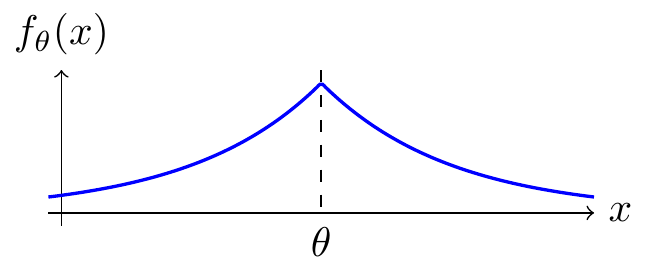
Example 30.4 (Double exponential location MLE) Let $X_1, \dots, X_n$ be i.i.d. random variables with PDF \[ f_\theta(x) = \frac{1}{2} e^{-|x - \theta|}. \tag{30.7}\] This PDF is shown below. This distribution is called the double exponential (or Laplace) distribution because it consists of two exponential distributions, one to either side of $\theta$.

Figure 30.1: PDF of the double exponential distribution $f_\theta(x) = \frac{1}{2} e^{-|x - \theta|}$.

To find the MLE of the location parameter $\theta$, we start by writing the likelihood for observed data $x_1, \ldots, x_n$: \[ L(\theta) = \frac{1}{2} e^{-|x_1 - \theta|} \dots \frac{1}{2} e^{-|x_n - \theta|} = \frac{1}{2^n} e^{-\sum_{i=1}^n |x_i - \theta|}. \]

The corresponding log-likelihood is \[ \ell(\theta) = \log L(\theta) = -n \log 2 -\sum_{i=1}^n |x_i - \theta|. \] We can maximize $\ell(\theta)$ or equivalently minimize \[ J(\theta) = \sum_{i=1}^n |x_i - \theta|. \tag{30.8}\]

However, we cannot take derivatives here because the absolute value function is not differentiable. This is illustrated in the code below, which shows that $J(\theta)$ is not differentiable at its minimizer (here, $\theta = 3$).

How do we minimize functions like these? We need to resort to other tricks. First, we sort the data so that \[ x_{(1)} \leq x_{(2)} \leq \dots \leq x_{(n-1)} \leq x_{(n)}. \] (These are called the order statistics of the data, whose properties we will study in Chapter 40.) Next, we pair the smallest observation with the largest and consider minimizing \[ |x_{(1)} - \theta| + |x_{(n)} - \theta|. \tag{30.9}\] Equation 30.9 represents the sum of the distances from $\theta$ to each observation. If $\theta$ is anywhere between $x_{(1)}$ and $x_{(n)}$, then the sum is constant, equal to the distance between the observations: $x_{(n)} - x_{(1)}$. This is also the minimum value; if $\theta$ is not between $x_{(1)}$ and $x_{(n)}$, then the distance between $\theta$ and just one of the observations will exceed $x_{(n)} - x_{(1)}$. This is illustrated in blue in Figure 30.2.

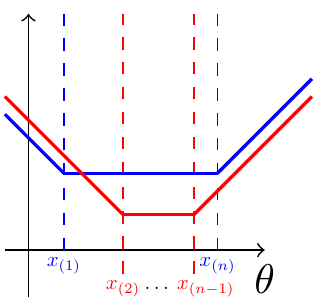
Figure 30.2: Graph of $|x_{(1)} - \theta| + |x_{(n)} - \theta|$ (blue) and $|x_{(2)} - \theta| + |x_{(n-1)} - \theta|$ (red) as a function of $\theta$.

Now, consider the next smallest value $x_{(2)}$ and the next largest value $x_{(n-1)}$. We can repeat the above argument to conclude that the minimum value of \[ |x_{(2)} - \theta| + |x_{(n-1)} - \theta| \] is achieved when $\theta$ is anywhere between $x_{(2)}$ and $x_{(n-1)}$. This is shown in red in Figure 30.2. Note that this choice of $\theta$ is also between $x_{(1)}$ and $x_{(n)}$, so it automatically minimizes Equation 30.9 as well.

We can repeat the same argument over and over, working our way inwards. If $n$ is even, then we will eventually reach \[ |x_{(n/2)} - \theta| + |x_{(n/2+1)} - \theta|, \] which is minimized when $\theta$ is anywhere between $x_{(n/2)}$ and $x_{(n/2+1)}$. Any such value of $\theta$ will simultaneously minimize all of the preceding pairs of terms and therefore minimize \[ \sum_{i=1}^n |x_i - \theta| = \underbrace{|x_{(1)} - \theta| + |x_{(n)} - \theta|}_{\text{minimized for any $x_{(1)} \leq \theta \leq x_{(n)}$}} + \underbrace{|x_{(2)} - \theta| + |x_{(n-1)} - \theta|}_{\text{minimized for any $x_{(2)} \leq \theta \leq x_{(n-1)}$}} + \dots + \underbrace{|x_{(n/2)} - \theta| + |x_{(n/2+1)} - \theta|}_{\text{minimized for any $x_{(n/2)} \leq \theta \leq x_{(n/2+1)}$}}. \]

Any value $\hat\theta \in [x_{(n/2)}, x_{(n/2+1)}]$ is the MLE and is called a sample median of the data. However, it is customary to define the sample median to be the midpoint of this interval—that is, \[ \hat\theta = \frac{x_{(n/2)} + x_{(n/2+1)}}{2} \text{ when $n$ is even}. \] Exercise 30.7 asks you to consider what happens when $n$ is odd.

Example 30.4 demonstrated two important lessons:

The MLE cannot always be obtained by blindly taking derivatives.
The MLE is not necessarily unique. There may be multiple values of $\theta$ that maximize the likelihood.

The minimizers of Equation 30.4 and Equation 30.8 are also useful in their own right.

The sample mean is the value of $c$ that minimizes the sum of squared distances to the data $\sum_{i=1}^n (x_i - c)^2$.
The sample median is the value of $c$ that minimizes the sum of absolute distances to the data $\sum_{i=1}^n |x_i - c|$.

30.3 Invariance of the MLE

In Example 30.3, we showed that the MLE of the normal variance $\sigma^2$ is \[ \widehat{\sigma^2} = \frac{1}{n} \sum_{i=1}^n (x_i - \hat\mu)^2. \] But what if we wanted the MLE of the standard deviation $\sigma$?

One option is to restart from scratch: write the likelihood in terms of $\sigma$, take the derivative, set it equal to zero, and solve for $\sigma$. However, there is a shortcut because the MLE obeys an invariance property: if you know the MLE for a parameter, the MLE for any function of that parameter is simply that function applied to your estimate.

Theorem 30.1 (Invariance Property of the MLE) Let $\hat\theta$ be the MLE of $\theta$, and let $g$ be a one-to-one function. Then, the MLE of $\phi = g(\theta)$ is \[ \hat\phi = g(\hat\theta). \tag{30.10}\]

Proof

Let $L(\theta)$ be the likelihood as a function of $\theta$. Then, the likelihood as a function of $\phi$ is \[ \tilde L(\phi) = L(g^{-1}(\theta)), \] where $g^{-1}$ is well-defined on the range of $g$ (because $g$ is one-to-one).

Now, let $\hat\phi = g(\hat\theta)$. Then, for any value of $\phi$, \[ \tilde L(\hat\phi) = L(g^{-1}(\hat\phi)) = L(\hat\theta) \geq L(g^{-1}(\phi)) = \tilde L(\phi), \] where the inequality follows because $\hat\theta$ is the MLE and therefore maximizes $L$.

By Theorem 30.1, the MLE of $\sigma = \sqrt{\sigma^2}$ must be \[ \hat\sigma = \sqrt{\widehat{\sigma^2}} = \sqrt{\frac{1}{n} \sum_{i=1}^n (x_i - \hat\mu)^2}. \tag{30.11}\]

Intuitively, if the likelihood is rewritten in terms of $\sigma$, the values of the likelihood do not change—only their locations do. The MLE of $\sigma^2$ is the location of the maximum value $L_{\text{max}}$, as shown on the left side of Figure 30.3. The MLE of $\sigma$ is the location of the same value after the transformation.

Figure 30.3: The invariance property: if $\widehat{\sigma^2}$ maximizes the likelihood for $\sigma^2$, then $\hat\sigma = \sqrt{\widehat{\sigma^2}}$ maximizes the likelihood for $\sigma$.

The invariance property guarantees that $\widehat{\sigma^2}$ (MLE of $\sigma^2$) and $\hat\sigma^2$ (square of the MLE of $\sigma$) are the same estimator, which allows us to use the two notations interchangeably.

30.4 Exercises

Exercise 30.1 (The likelihood principle) Your friend claims to be an excellent free throw shooter. You would like to estimate the probability $p$ that they make a free throw. Assume that free throws are independent.

Suppose they take 16 shots and successfully make 10. Write down the likelihood function $L_{X=10}(p)$.
Suppose they take as many shots as necessary until they successfully make 10 free throws. Suppose that it takes $Y=16$ free throws. Write down the likelihood function $L_{Y=16}(p)$.

The two likelihood functions above are different, but they are related. How are they related? Why does this imply that the MLE of $p$ is the same in both cases? Calculate the MLE of $p$.

Even though the two likelihood functions are different, they both lead to the same inference about $p$. This is an example of the likelihood principle.

Exercise 30.2 (Poisson MLE) During World War II, the Germans fired V-1 flying bombs at London. Some people suspected that the Germans were aiming at specific targets, while others argued that the bombs were striking random targets.

To answer this question, Clarke (1946) divided South London into a grid of 576 squares, each of $0.25$ square kilometers, and counted the V-1 number of flying bombs that landed in each square. His data is shown in the table below:

Number of bombs ($k$)	0	1	2	3	4	5	Total
Squares with $k$ bombs	229	211	93	35	7	1	576

If the bombs were dropped at random, then the counts $X_1, X_2, \dots, X_{576}$ should be i.i.d. $\text{Poisson}(\mu)$ random variables.

Graph the likelihood as a function of $\mu$ for the above data.
Calculate the MLE of $\mu$.
Plot the estimated Poisson PMF on top of the observed frequencies. Does it seem reasonable to assume the bombs were dropped at random?

Exercise 30.3 (Rayleigh distribution) The data set (https://dlsun.github.io/skis/data/wind.csv) contains daily average wind speeds for 1961-1978 at 12 stations in Ireland. (Haslett and Raftery 1989) We will look at the average wind speed on the first day of each month in Kilkenny.

One common model for wind speed is the Rayleigh distribution. Exercise 38.7 provides a physical motivation for this distribution. Let $X_1, \dots, X_n$ be the wind speeds, and suppose that they are a random sample from a Rayleigh distribution with unknown parameter $\sigma^2$: \[ f_{\sigma^2}(x) = \begin{cases} \frac{x}{\sigma^2} e^{-\frac{x^2}{2\sigma^2}} & x \geq 0 \\ 0 & \text{otherwise} \end{cases}. \tag{30.12}\]

Graph the likelihood as a function of $\sigma^2$ for the Kilkenny data.
Find the MLE of $\sigma^2$.
Why do you think we took the average wind speeds on the first day of each month, rather than all of the daily average wind speeds?

Exercise 30.4 (Power distribution) Let $X_1, \dots, X_n$ be i.i.d. with PDF \[ f(x) = \begin{cases} (\theta + 1)x^\theta & 0 \leq x \leq 1 \\ 0 & \text{otherwise} \end{cases}, \] where $\theta$ is unknown. Find the MLE of $\theta$.

Exercise 30.5 (Uniform distribution) Let $X_1, \dots, X_n$ be a random sample from a $\text{Uniform}(0,\theta)$ distribution, where the upper bound $\theta$ is unknown. Find the MLE of $\theta$.

Exercise 30.6 (Exponential location MLE) Let $X_1, \dots, X_n$ be i.i.d. with PDF \[ f_\theta(x) = \begin{cases} e^{-(x - \theta)}, & x \geq \theta, \\ 0, & x < \theta. \end{cases} \tag{30.13}\] What is the MLE of $\theta$?

Hint: What happens to the likelihood when $\theta$ is greater than $\min(X_1, \dots, X_n)$?

Exercise 30.7 (Double exponential MLE when $n$ is odd) In Example 30.4, we showed that when $n$ is even, the MLE of $\theta$ can be any value between $x_{(n/2)}$ and $x_{(n/2+1)}$.

What is the MLE of $\theta$ when $n$ is odd? Is the MLE unique?

Exercise 30.8 (MLE of the exponential mean) Let $X_1, \dots, X_n$ be i.i.d. $\text{Exponential}(\lambda)$. What is the MLE of $\mu \overset{\text{def}}{=}\text{E}\!\left[ X_1 \right]$?