48  Bayesian Statistics

$$

$$

So far, we have adopted a frequentist approach to statistical inference. That is, the parameter \(\theta\) is unknown, but it is a fixed quantity. The randomness is only in the data \(X_1, \dots, X_n\).

The Bayesian approach is an alternative framework, which assumes that the parameter \(\theta\) is also a random variable. This chapter provides an overview of the Bayesian approach.

48.1 From the Prior to the Posterior

The Bayesian approach starts by assuming a distribution for the parameter, called the prior distribution.

To be concrete, consider Example 29.4, where we want to estimate \(p\), the probability of rolling a six with a skew die. A Bayesian would start with a prior distribution on \(p\), reflecting their belief about how likely different values of \(p\) are. Since \(p\) takes on values between \(0\) and \(1\), it is reasonable to model \(p\) using a \(\text{Beta}(\alpha, \beta)\) distribution, which has PDF \[ \pi(p) = \frac{\Gamma(\alpha +\beta)}{\Gamma(\alpha) \Gamma(\beta)} p^{\alpha - 1} (1 - p)^{\beta - 1}; \qquad 0 < p < 1. \tag{48.1}\] (The Bayesian would need to specify the values of \(\alpha\) and \(\beta\), which are called hyperparameters. For example, a choice of \(\alpha = \beta = 1\) would correspond to a uniform distribution.)

Next, the Bayesian updates their belief in response to the observed data \(X\). That is, they determine the distribution of \(p \mid X\), called the posterior distribution. The key ingredient is Bayes’ rule (Proposition 26.2), which gives this approach its name.

Example 48.1 (Calculating the posterior distribution of \(p\)) Suppose we roll the skew die \(n\) times and observe \(x\) sixes. By Bayes’ rule (Proposition 26.2), the posterior distribution of \(p\), given this information, has PDF \[ \begin{align*} \pi(p \mid x) &= \frac{\pi(p) f(x \mid p)}{ f_X(x) } \\ &= \frac{\frac{\Gamma(\alpha +\beta)}{\Gamma(\alpha) \Gamma(\beta)} p^{\alpha-1} (1-p)^{\beta-1} \cdot \binom{n}{x} p^x (1-p)^{n-x}}{ f_X(x) } \end{align*} \]

Notice that the denominator does not depend on \(p\). In other words, for the purposes of determining the posterior, it is just a constant that makes the PDF integrate to 1. We will absorb this constant, as well as others that do not depend on \(p\), into a term \(C_x\): \[ \begin{align*} \pi(p \mid x) &= C_x \cdot p^{\alpha-1} (1-p)^{\beta-1} \cdot p^x (1-p)^{n-x} \\ &= C_x \cdot p^{\alpha + x - 1} (1 - p)^{\beta + n - x - 1}. \end{align*} \]

We recognize this posterior as the PDF of a \(\text{Beta}(\alpha+x, \beta+n-x)\) distribution. In hindsight, this means the constant must be \[ C_x = \frac{\Gamma(\alpha + \beta + n)}{\Gamma(\alpha + x) \Gamma(\beta + n - x)}. \] When the posterior is a named distribution, we can safely ignore “constants” that do not depend on the parameter until the very end. This is another reason it is convenient to choose a beta prior; it guarantees that the posterior will also be beta.

To see how this works in practice, suppose that Barry the Bayesian believes that the die is likely fair (or close to it). He chooses a \(\text{Beta}(\alpha=2, \beta=10)\) prior for \(p\). After observing \(X = 7\) sixes in \(n = 25\) rolls, Example 48.1 says that he should update his belief to a \(\text{Beta}(\alpha=2 + 7, \beta=10 + 18)\) distribution. These prior and posterior distributions are shown in blue below. Notice how the prior (solid) is centered around \(\frac{\alpha}{\alpha + \beta} = \frac{1}{6}\), but the posterior (dashed) is shifted toward the observed data (\(\frac{7}{25} = 0.28\)).

To understand why the Bayesian approach is controversial, consider another Bayesian statistician, Agnes the Agnostic, who has no opinion about whether or not the die is fair. She instead chooses a uniform prior (i.e., \(\text{Beta}(\alpha=1, \beta=1)\)) for \(p\). After observing \(X = 7\) sixes in \(n=25\) rolls, her posterior is a \(\text{Beta}(\alpha=1 + 7, \beta=1 + 18)\) distribution. These prior and posterior distributions are shown in orange above.

In the Bayesian approach, the posterior captures everything there is to know about a parameter. Therefore, it is troubling that Agnes and Barry could end up with different posterior distributions after observing the same data, simply because they had different prior beliefs. This subjectivity makes the Bayesian approach suspect to some statisticians.

In the remaining sections, we will explore the Bayesian analogs of point and interval estimation. Both use the posterior distribution as a starting point.

48.2 Bayesian Estimation

In Example 29.4, we saw that a frequentist would estimate \(p\) by the MLE. How would a Bayesian reduce the posterior distribution to a single estimate?

One obvious idea is to take the value of \(p\) that maximizes the PDF of the posterior distribution, or posterior mode. In Exercise 41.3, we derived the mode of a beta distribution. Applying that result to the posterior distribution in Example 48.1, we see that the posterior mode is \[ \text{MAP} = \frac{\alpha + X - 1}{\alpha + \beta + n - 2}. \] This is called the maximum a posteriori (MAP) estimator.

Although the MAP estimator is not bad, it is usually not the best estimator. The next theorem justifies why Bayesians typically prefer the posterior mean.

Theorem 48.1 (Posterior mean minimizes Bayes MSE) The posterior mean \(\text{E}\!\left[ \theta\mid X \right]\) is the estimator \(\hat\theta\) that minimizes \[ \text{E}\!\left[ (\hat\theta - \theta)^2 \right], \tag{48.2}\] where the expectation is taken over both \(\hat\theta\) and \(\theta\).

Proof

Remember that an estimator \(\hat\theta\) is just a function of the data \(g(X)\). By Proposition 27.4, the function \(g(X)\) that minimizes \[ \text{E}\!\left[ (g(X) - \theta)^2 \right] \] is \(\text{E}\!\left[ \theta \mid X \right]\).

Note that Equation 48.2 is distinct from the (frequentist) MSE in Definition 32.2. There, \(\theta\) was regarded as fixed, and the expectation was only taken over the estimator \(\hat\theta\). In Equation 48.2, \(\theta\) is regarded as random, and the expectation is taken over \(\theta\) as well as the estimator \(\hat\theta\).

Now, we apply Theorem 48.1 to Example 48.1 and determine the Bayesian estimator of \(p\).

Example 48.2 (Posterior mean of \(p\)) In Example 48.1, we determined the posterior distribution to be \[ p \mid X=x \sim \text{Beta}(\alpha+x, \beta+n-x), \] so the posterior mean is \[ \text{E}\!\left[ p \mid X \right] = \frac{\alpha + X}{\alpha + X + \beta + n - X} = \frac{\alpha + X}{\alpha + \beta + n} \tag{48.3}\] by Proposition 41.2. In other words, the Bayes estimator simply adds \(\alpha\) successes and \(\beta\) failures to the observed data, where \(\alpha\) and \(\beta\) come from the prior.

Agnes, who chose a prior of \(\alpha = \beta = 1\), would estimate \(p\) as \[ \hat p_A = \frac{1 + 7}{2 + 25} = \frac{8}{27} \approx 0.286, \] while Barry, who chose a prior of \(\alpha = 2, \beta = 10\), would estimate \(p\) as \[ \hat p_B = \frac{2 + 7}{12 + 25} = \frac{9}{37} \approx 0.257. \] Once again, we see that two Bayesians can end up with different answers if they start with different prior beliefs.

Notice that we can express Equation 48.3 as a weighted average of the prior mean and the MLE: \[ \text{E}\!\left[ p \mid X \right] = \underbrace{\frac{\alpha + \beta}{\alpha + \beta + n}}_{1-w} \underbrace{\frac{\alpha}{\alpha + \beta}}_{\text{E}\!\left[ p \right]} + \underbrace{\frac{n}{\alpha + \beta + n}}_{w} \underbrace{\frac{X}{n}}_{\hat p_{\text{MLE}}}. \tag{48.4}\] Since \(\hat p_{\text{MLE}}\) is unbiased, this shows that the posterior mean is generally biased, shrunken toward the prior mean. Even Agnes the Agnostic, who tried to make “no” assumptions about \(p\) by choosing a uniform prior, ended up with an estimator that is shrunken toward the prior mean of \(0.5\). In the words of the statistician R. A. Fisher, “Thinking that you don’t know and thinking that the probabilities of all the possibilities are equal is not the same thing.” (McGrayne 2011) It is impossible to be truly agnostic in a Bayesian analysis.

However, as more data is collected (\(n\to\infty\)), the weight on the prior in Equation 48.4 decreases to \(0\). That is, there is very little difference between \(\text{E}\!\left[ p \mid X \right]\) and \(\hat p_{\text{MLE}}\) when \(n\) is large. This also means that Agnes and Barry’s estimates will converge to the same value as \(n\) increases.

48.3 Credible Intervals

In Chapter 47, we saw that a frequentist would quantify their uncertainty about a parameter \(\theta\) using a confidence interval. Because \(\theta\) is not random, the interpretation of the confidence interval required some finesse. By contrast, the Bayesian regards \(\theta\) as random, so their uncertainty about \(\theta\) should be baked into the posterior distribution. Therefore, the Bayesian analog of the confidence interval is any interval that has 95% probability under the posterior. Such an interval is called a credible interval.

To be precise, a 95% credible interval is an interval \(C(\vec X)\) such that \[ P(\theta \in C(\vec X) \mid \vec X) = 0.95. \tag{48.5}\] A frequentist could never make this statement because the only quantity that is random in their world is \(\vec X\). If we condition on \(\vec X\), then nothing is random. Contrast Equation 48.5 with the definition of a confidence interval (Equation 47.3). A Bayesian is only able to make a statement such as Equation 48.5 because they are willing to assume that \(\theta\) is also random.

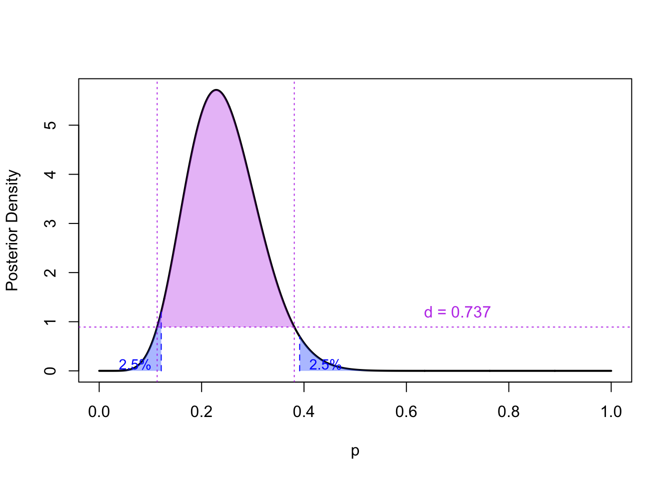
How do we construct a credible interval \(C(\vec X)\)? The simplest way is to lop equal tails (i.e., 2.5%) off each end of the posterior. Another method, which is more principled but requires more computation, is to take the parameter values with the highest posterior density until the region has 95% probability under the posterior. The two methods will agree when the posterior is symmetric and unimodal, but will be different in general, as illustrated in Figure 48.1.

Figure 48.1: Posterior distribution with equal-tail (blue) and highest posterior density (purple) 95% credible intervals.

Example 48.3 (Credible intervals for \(p\)) We will calculate credible intervals based on Barry’s prior of \(\text{Beta}(\alpha=2, \beta=10)\). Recall from Example 48.1 that his posterior is \(\text{Beta}(9, 28)\).

To obtain the equal-tail credible interval, we simply look up the quantiles of this beta distribution.

To obtain the highest posterior density interval, we first need a function that finds the values of \(p\) where the posterior density equals a level \(d\).

Next, we find the value of \(d\) which yields 95% probability.

The 95% credible intervals for \(p\) obtained from the two approaches are:

• Equal-tail: \([0.121, 0.391]\)
• Highest Posterior Density: \([0.113, 0.381]\).

Both credible intervals have 95% probability under the posterior distribution, but the highest posterior density interval is usually the shortest interval with this property (at the cost of more computation).

48.4 Exercises

Exercise 48.1 (Comparing credible and confidence intervals) Calculate the 95% credible intervals (using the two approaches) for Agnes. Compare these intervals with the confidence interval for \(p\) in Example 47.4, which was \([0.143, 0.476]\).

Exercise 48.2 (Normal prior) Suppose we observe \(X_1, \dots, X_n \sim \text{Normal}(\mu, \sigma^2)\), where \(\sigma^2\) is known and the goal is to estimate \(\mu\). We will assume a prior of the form \[ \mu \sim \text{Normal}(\mu_0, \tau^2). \]

1. Determine the posterior distribution \(\mu \mid X_1, \dots, X_n\).
2. Determine the posterior mean \(\text{E}\!\left[ \mu\mid X_1, \dots, X_n \right]\). How does this posterior mean compare with the MLE as \(n\to\infty\)? (Hint: Try to come up with a representation like Equation 48.4 for the posterior mean.)
3. Calculate a 95% credible interval for \(\mu\). How does it compare with the 95% confidence interval in Proposition 47.1? (Hint: It does not matter which method you use to construct the credible interval because the posterior distribution should by symmetric and unimodal.)

McGrayne, Sharon Bertsch. 2011. The Theory That Would Not Die: How Bayes’ Rule Cracked the Enigma Code, Hunted down Russian Submarines, & Emerged Triumphant from Two Centuries of Controversy. Yale University Press.